Abstract

Twisted bilayer graphene (TBG) is a recently discovered two-dimensional superlattice structure which exhibits strongly-correlated quantum many-body physics, including strange metallic behavior and unconventional superconductivity.

扭曲双层石墨烯(TBG)是最近发现的一种二维超晶格结构, 它表现出强相关量子多体物理学, 包括奇异的金属行为和非常规超导性.

Most of TBG exotic properties are connected to the emergence of a pair of isolated and topological flat electronic bands at the so-called magic angle, $\theta \approx 1.05°$, which are nevertheless very fragile.

TBG 的大部分奇异特性都与在所谓的魔角 $\theta \approx 1.05°$ 处出现的一对孤立的拓扑平坦电子带有关, 但这些电子带非常脆弱.

In this work, we show that, by employing chiral optical cavities, the topological flat bands can be stabilized away from the magic angle in an interval of approximately $0.8° < \theta < 1.3°$.

在这项工作中, 我们展示了通过采用手性光腔, 拓扑平坦带可以稳定在大约 $0.8° < \theta < 1.3°$ 的魔幻角范围内.

As highlighted by a simplified theoretical model, time reversal symmetry breaking, induced by the chiral nature of the cavity, plays a fundamental role in flattening the isolated bands and gapping out the rest of the spectrum.

The efficiency of the cavity is discussed as a function of the twisting angle, the light-matter coupling and the optical cavity characteristic frequency.

Our results demonstrate the possibility of engineering flat bands in TBG using optical devices, extending the onset of strongly-correlated topological electronic phases in Moir ́e superlattices to a wider range in the twisting angle.

正如一个简化的理论模型所强调的那样, 空腔的手性所引起的 时间反演对称性破坏, 在使孤立的能带平坦化和将光谱的其余部分隔开方面起着根本性的作用.

我们讨论了腔体效率与扭转角、光物质耦合和光腔特征频率的函数关系.

我们的研究结果证明了利用光学器件在 TBG 中设计平坦带的可能性, 并将 Moir ́e 超晶格中强相关拓扑电子相的发生扩展到更宽的扭转角范围.

Introduction

Controlling and engineering quantum phases of matter is a central task in condensed matter physics. Inspired by the original discovery of singlelayer graphene, two-dimensional (2D) materials have emerged as a versatile platform to realize stronglycorrelated physics in quantum many body systems.

控制和设计物质的量子相是凝聚态物理学的一项核心任务. 受最初发现单层石墨烯的启发, 二维(2D)材料已成为实现量子多体系统中强相关物理学的多功能平台.

Recently, unconventional superconductivity was discovered in twisted bilayer graphene (TBG), a two dimensional superlattice where one layer of graphene is stacked on top of another at a special magic twisting angle, i.e., $\theta \approx 1.05°$.

最近, 在扭曲双层石墨烯(TBG)中发现了非常规超导电性, 在这种二维超晶格中, 一层石墨烯以一个特殊的魔力扭曲角度(即 $\theta \approx 1.05°$)堆叠在另一层石墨烯之上.

Galvanized by this breakthrough, several other stacked two-dimensional systems that host exotic superconductivity, such as twisted multilayer graphene, have been revealed.

While the underneath physical mechanism of superconductivity in twisted 2D systems is still under debate, it is clear that the isolated electronic flat band appearing at the magical angle plays an essential role.

Besides superconductivity, flat bands are also indispensable for the emergence of strongly-correlated insulating states and the strangemetal phase near the superconducting dome in the phase diagram of TBG, which closely mimics that of cuprate superconductors.

在这一突破的推动下, 其他几种蕴含奇异超导性的叠层二维系统(如扭曲多层石墨烯)也被揭示出来.

虽然人们对扭曲二维系统超导的基本物理机制仍有争议, 但在神奇角度出现的孤立电子平带显然起着至关重要的作用.

除了超导性之外, 平带对于 TBG 相图中强相关绝缘态和超导穹顶附近的奇异金属相的出现也是不可或缺的, 这与杯状超导体的相图非常相似.

However, despite being a promising platform for studying strongly correlated physics, the unavoidable and uncontrollable non-uniformity of the twist angle across the sample, and the consequent difficulty in keeping the twist angle at its magic value, prevented a wide realization of these phenomena.

然而, 尽管这是研究强相关物理学的一个很有前途的平台, 但由于整个样品的扭转角存在不可避免和不可控制的不均匀性, 因此很难将扭转角保持在其奇异值上, 这就阻碍了这些现象的广泛实现.

More precisely, because the magical-angle configuration is unstable, a little offset (around $±0.1°$) of the twisting angle easily destroys all the emergent exotic properties of TBG.

更确切地说, 由于魔转角构型不稳定, 扭转角度稍有偏移(约为±0.1°)就会轻易破坏 TBG 的所有新奇特性.

In this regard, one of the most important challenges in the field is therefore to achieve superconductivity at non-magic values of the twisting angle. To achieve this final goal, it is desirable to realize a primary step, namely to create and stabilize electronic flat bands in a wider range of the twisting angle.

因此, 该领域最重要的挑战之一就是在非神奇的扭转角值下实现超导. 为了实现这一最终目标, 最好能实现更基础的一步, 也就是在更大的扭转角范围内创建并稳定电子平带.

In this Letter, we propose a new method to engineer stable flat bands at non-magic angles by embedding twisted-bilayer graphene in a vacuum chiral cavity (see top panel in Figure 1 for a cartoon of the setup). Using vacuum cavities to control materials and molecules has emerged as a fruitful playground connecting quantum optics to condensed matter and chemistry.

在本篇快报中, 我们提出了一种新方法: 将扭曲的双层石墨烯嵌入真空手性腔(见图 1 顶部面板中的设置示意图), 从而在非魔转角下设计出稳定的平带. 利用抽真空的空腔来控制材料和分子, 这种方法已成为贯通量子光学与凝聚态物质/化学的一个富有成效的途径.

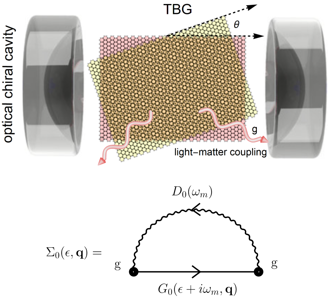
Top panel. A cartoon of the optical setup considered in this work. Two skewed sheets of graphene are stacked on top of each other with a twisting angle $\theta$ creating a characteristic Moir ́e pattern. They are then put inside a chiral optical cavity with a light-matter coupling $g$ and a characteristic frequency $\omega_{c}$. Bottom panel. The dominant Feynman diagram describing light-matter interaction in the optical chiral cavity and giving rise to the self-energy $\Sigma_{0}(\epsilon,\mathbf{q})$.

上半部分. 本研究中使用的光学装置示意图. 两片歪斜的石墨烯叠放在一起, 扭转角度为 $\theta$, 形成特征性的 Moir ́e 图案. 然后将它们放入一个手性光腔中, 光-物质耦合度为 $g$, 特征频率为 $\omega_{c}$. 下半部分. 描述光学手性腔中光与物质相互作用并产生自能 $\Sigma_{0}(\epsilon,\mathbf{q})$ 的主要费曼图。

Vacuum cavity engineering is superior to the Floquet method, where external electromagnetic radiation drives the system out of equilibrium, since this second route inevitably heats up the system, destroying quantum coherence and inducing transient phenomena away from thermal equilibrium states.

真空空腔工程优于弗洛凯方法, 后者是通过外部电磁辐射使系统脱离平衡状态, 然而第二种途径不可避免地加热系统, 破坏量子相干性, 诱发脱离热平衡状态的瞬态现象.

In the past, the usage of vacuum cavities has been proposed to design material conductivity, unconventional superconductivity, topological properties, and even chemical reactivity. Some of these proposals have been already successfully realized experimentally.

过去, 曾有人提出利用真空腔体来设计材料的导电性、非传统超导性、拓扑特性, 甚至化学反应性. 其中的一些建议已经在实验中成功实现.

A fundamental property of vacuum chiral cavities is that time-reversal symmetry is broken without the need of an external driving.

Time-reversal symmetry breaking is essential since, as we will see, quantum fluctuations alone can not significantly influence the electronic bands in TBG.

In single-layer graphene, a band gap can be induced by quantum fluctuations in a chiral cavity as well.

真空手性空腔的一个基本特性是, 无需外部驱动即可打破时间反演对称性.

时间反演对称性的破缺至关重要, 因为正如我们将看到的那样, 仅靠量子波动并不能显著影响 TBG 中的电子带.

在 单层石墨烯 中, 手性腔中的量子波动也能诱发带隙.

However, the effect is too small to be directly observed due to the large bandwidth.

As we will demonstrate, the situation is different in TBG near the magic angle, where the small bandwidth enables time-reversal symmetry-broken quantum fluctuations to play a significant role.

然而, 由于带宽太大, 这种效应太小, 无法直接观测到.

正如我们将证明的那样, 在魔转角附近的 TBG 中情况有所不同, 那里的小带宽使时间反转对称破缺的量子波动发挥了重要作用.

In recent years, a number of works have realized the vital impact of symmetry breaking on quantumfluctuations-related phenomena, such as anomalous Casimir effects, topological gap generation, and selection of chiral molecules in chemical reactions.

A recent work by one of us highlighted the combined power of symmetry breaking and quantum fluctuations, proving that symmetry breaking effects can be transmitted from a material to its vicinity by vacuum quantum fluctuations.

In this scenario, the vacuum in proximity of a material with broken symmetries is referred to as its Quantum Atmosphere.

近年来, 许多研究已经意识到对称性破缺对量子波动相关现象的重要影响, 如反常卡西米尔效应、拓扑间隙的产生、化学反应中手性分子的选择等.

我们其中一人最近的一项研究强调了对称性破缺与量子波动的结合的威力, 证明了对称性破缺效应可以通过真空量子波动从材料传递到其附近.

在这种情况下, 具有对称性破缺的材料附近的真空被称为材料的 量子大气.

In this Letter, we investigate the band renormalization of TBG in the time-reversal symmetry broken quantum atmosphere provided by a chiral cavity.

We start from a faithful tight-binding model of TBG and calculate the one-loop self-energy induced by the light-matter coupling. The bottom panel of Figure 1 displays the specific Feynman diagram considered.

We find that, for experimentally realizable values of the light-matter coupling and cavity frequency, the topological flat bands in TBG can be stabilized away from the magic angle in an interval of approximately $0.8° < \theta < 1.3°$.

Our derivation and calculations can be directly generalized to other twisted 2D systems.

在这封快报中, 我们研究了手性腔提供的时间反演对称破缺量子环境中 TBG 的带重正化.

我们从 TBG 的经典的紧束缚模型出发, 计算光-物质耦合引起的 one loop 自能量. 图 1 底部显示了所考虑的具体费曼图.

我们发现, 对于光-物质耦合和空腔频率的实验可实现值, TBG 中的拓扑平坦带可以稳定地偏离魔转角, 其区间大约为 $0.8° < \theta < 1.3°$.

我们的推导和计算可直接推广到其他扭曲的二维系统.

Setup & methods

To set the stage, we model the Hamiltonian of the combined system, TBG and cavity, as follows:

$$ \hat{H} = \hat{H}_{\text{TBG}}\left(\mathbf{q} - e\hat{\mathbf{A}}\right) + \hbar\omega_{c}\hat{a}^{\dagger}\hat{a} $$

where $\hat{H}_{\text{TBG}}$ represents the TBG Hamiltonian in reciprocal space, and $\omega_{c}$ is is the cavity photonic mode frequency.

为了做好铺垫, 我们对 TBG 和空腔组合系统的哈密顿建立如下模型：

$$ \hat{H} = \hat{H}_{\text{TBG}}\left(\mathbf{q} - e\hat{\mathbf{A}}\right) + \hbar\omega_{c}\hat{a}^{\dagger}\hat{a} $$

其中, $\hat{H}_{text{TBG}}$ 表示动量空间中 TBG 的哈密顿, $\omega_{c}$ 是指空腔光子模式频率.

TBG and cavity photonic modes are coupled through Peierls substitution $\mathbf{q}\rightarrow \mathbf{q} - e\hat{\mathbf{A}}$, where $\hat{\mathbf{A}}$ can be expressed in terms of photonic creation and annihilation operators, i.e., $\hat{\mathbf{A}} = A_{0}(\epsilon^{*}\hat{a}^{\dagger} + \epsilon\hat{a})$.

Here, $\epsilon$ is the polarization tensor of the cavity photonic modes and $A_{0} = \sqrt{\frac{\hbar}{2\epsilon_{0}V\omega_{c}}}$ is the mode amplitude in terms of the cavity volume $V$.

We focus on chiral cavities where the photonic polarization is given by $\epsilon = \frac{1}{\sqrt{2}}(\mathbf{e}_{\text{x}} + i\mathbf{e}_{\text{y}})$, with $\mathbf{e}_{\text{x}(\text{y})}$ the unit vector in the $x(y)$-direction. Our setup can be straightforwardly generalized to the multi-mode case.

TBG 和腔体光子模通过 Peierls 置换 耦合为 $\mathbf{q}\rightarrow \mathbf{q} - e\hat{\mathbf{A}}$, 其中 $\hat{\mathbf{A}}$ 可以用光子创造和湮灭算子来表示, 即, $\hat{\mathbf{A}} = A_{0}(\epsilon^{*}\hat{a}^{\dagger} + \epsilon\hat{a})$.

这里, $\epsilon$ 是空腔光子模式的极化张量, $A_{0} = \sqrt{\frac{\hbar}{2\epsilon_{0}V\omega_{c}}}$ 是以空腔体积 $V$ 项表示的模式振幅.

To be concrete, let us consider the effective tightbinding Hamiltonian $\hat{H}_{\text{TBG}}(\mathbf{q})$:

$$ \left(\begin{array}{ccccc} H_{1}(\mathbf{q}) & T_{\mathbf{q}_{b}} & T_{\mathbf{q}_{tr}} & T_{\mathbf{q}_{tl}} & \dots \\ T_{\mathbf{q}_{b}}^{\dagger} & H_{2}(\mathbf{q}-\mathbf{q}_{b}) & 0 & 0 & \dots \\ T_{\mathbf{q}_{tr}}^{\dagger} & 0 & H_{2}(\mathbf{q}-\mathbf{q}_{tr}) & 0 & \dots \\ T_{\mathbf{q}_{tl}}^{\dagger} & 0 & 0 & H_{2}(\mathbf{q}-\mathbf{q}_{tl}) & \dots \\ \vdots & \vdots & \vdots & \vdots & \ddots \end{array}\right) $$

where $\mathbf{q}$ is the wave-vector, and $H_{1,2}(\mathbf{q})$ indicate the Hamiltonian of the top/bottom layer respectively.

具体来说, 让我们考虑有效紧束缚哈密顿量 $\hat{H}_{\text{TBG}}(\mathbf{q})$：

$$ \left(\begin{array}{ccccc} H_{1}(\mathbf{q}) & T_{\mathbf{q}_{b}} & T_{\mathbf{q}_{tr}} & T_{\mathbf{q}_{tl}} & \dots \\ T_{\mathbf{q}_{b}}^{\dagger} & H_{2}(\mathbf{q}-\mathbf{q}_{b}) & 0 & 0 & \dots \\ T_{\mathbf{q}_{tr}}^{\dagger} & 0 & H_{2}(\mathbf{q}-\mathbf{q}_{tr}) & 0 & \dots \\ T_{\mathbf{q}_{tl}}^{\dagger} & 0 & 0 & H_{2}(\mathbf{q}-\mathbf{q}_{tl}) & \dots \\ \vdots & \vdots & \vdots & \vdots & \ddots \end{array}\right) $$

其中, $\mathbf{q}$ 是波矢, $H_{1,2}(\mathbf{q})$ 分别表示顶层/底层的哈密顿量.

Moreover, we have defined:

$$ \mathbf{q}_{b} = \frac{1}{3}(\mathbf{b}_{1}^{m} - \mathbf{b}_{2}^{m}),\quad\mathbf{q}_{tr} = \frac{1}{3}(\mathbf{b}_{1} + 2\mathbf{b}_{2}^{m}),\quad\mathbf{q}_{tl} = \frac{1}{3}(-2\mathbf{b}_{1}^{m} - \mathbf{b}_{2}^{m}) $$

where $\mathbf{b}_{1}^{m}$ and $\mathbf{b}_{2}^{m}$ are Moir ́e reciprocal vectors. The twisting angle $\theta$ is hidden in these vectors; see Fig.6.11 in Ref.[56] for more details.

此外, 我们还定义了

$$ \mathbf{q}_{b} = \frac{1}{3}(\mathbf{b}_{1}^{m} - \mathbf{b}_{2}^{m}),\quad\mathbf{q}_{tr} = \frac{1}{3}(\mathbf{b}_{1} + 2\mathbf{b}_{2}^{m}),\quad\mathbf{q}_{tl} = \frac{1}{3}(-2\mathbf{b}_{1}^{m} - \mathbf{b}_{2}^{m}) $$

其中 $\mathbf{b}_{1}^{m}$ 和 $\mathbf{b}_{2}^{m}$ 是 Moir ́e 倒易矢量. 扭转角 $\theta$ 隐藏在这些矢量中；详情请参见参考文献[56]中的图 6.11.

The hopping matrix elements are given by,

$$ T_{\mathbf{q}_{b}} = t\left(\begin{array}{cc} 1 & 1 \\ 1 & 1 \end{array}\right),\quad T_{\mathbf{q}_{tr}} = t\left(\begin{array}{cc} e^{i\phi} & 1 \\ e^{-i\phi} & e^{i\phi} \end{array}\right),\quad T_{\mathbf{q}_{tl}} = t\left(\begin{array}{cc} e^{-i\phi} & 1 \\ e^{i\phi} & e^{-i\phi} \end{array}\right) $$

where $\phi = 2\pi/3$ and $t = 0.11$ is the hopping parameter. For more details about the TBG Hamiltonian we refer to the Supplementary Information (SI).

跃迁矩阵元的表达式为

$$ T_{\mathbf{q}_{b}} = t\left(\begin{array}{cc} 1 & 1 \\ 1 & 1 \end{array}\right),\quad T_{\mathbf{q}_{tr}} = t\left(\begin{array}{cc} e^{i\phi} & 1 \\ e^{-i\phi} & e^{i\phi} \end{array}\right),\quad T_{\mathbf{q}_{tl}} = t\left(\begin{array}{cc} e^{-i\phi} & 1 \\ e^{i\phi} & e^{-i\phi} \end{array}\right) $$

其中, $\phi = 2\pi/3$ 和 $t = 0.11$ 是跳跃参数. 有关 TBG 哈密顿的更多细节, 请参阅补充信息(SI).

Once the effective Hamiltonian is known, the bare electron propagator can be obtained using

$$ G^{-1}(\epsilon,\mathbf{q}) = [(\epsilon + i0^{+})\mathbf{I} - H_{\text{TBG}}(\mathbf{q})]^{-1} $$

一旦知道了有效哈密顿量, 就可以用以下方法得到裸电子传播子:

$$ G^{-1}(\epsilon,\mathbf{q}) = [(\epsilon + i0^{+})\mathbf{I} - H_{\text{TBG}}(\mathbf{q})]^{-1} $$

The full electron propagator, taking into account the interaction with the vacuum cavity, can then be derived from the Dyson equation

$$ G^{-1}(\epsilon,\mathbf{q}) = G^{-1}_{0}(\epsilon,\mathbf{q}) - \Sigma_{0}(\epsilon,\mathbf{q}) $$

考虑到与真空空腔的相互作用, 完整的电子传播子可以从 戴森方程 中推导出来

$$ G^{-1}(\epsilon,\mathbf{q}) = G^{-1}_{0}(\epsilon,\mathbf{q}) - \Sigma_{0}(\epsilon,\mathbf{q}) $$

where $\Sigma_{0}$ is the self-energy (see bottom panel of Fig.1) given by

$$ \Sigma_{0}(\epsilon,\mathbf{q}) = -\frac{q^{2}}{\beta}\sum_{m = 1}^{\infty}G_{0}(\epsilon+i\omega_{m},\mathbf{q})D_{0}(\omega_{m}) $$

其中, $\Sigma_{0}$ 是自能(见图 1 底部面板), 其计算公式为

$$ \Sigma_{0}(\epsilon,\mathbf{q}) = -\frac{q^{2}}{\beta}\sum_{m = 1}^{\infty}G_{0}(\epsilon+i\omega_{m},\mathbf{q})D_{0}(\omega_{m}) $$

Here, $\omega_{m} = 2\pi mk_{B}T$ is the $m$th Matsubara frequency and $g = v_{F}eA_{0}$ denotes the electron-photon coupling strength with $v_{F}$ the Fermi velocity of monolayer graphene and $e$ the electromagnetic coupling.

Finally, $D_{0}(\omega_{m})$ is the photon propagator given by

$$ D_{0}(\omega_{m}) = \left(\begin{array}{ccc} \frac{-1}{i\omega_{m} + \omega_{c}} & 0 & \dots \\ 0 & \frac{1}{i\omega_{m} - \omega_{c}} & \dots \\ \vdots & \vdots & \ddots \end{array}\right) $$

with $\omega_{c}$ the cavity frequency.

这里, $\omega_{m} = 2\pi mk_{B}T$ 是第 $m$ 个 松原频率, $g = v_{F}eA_{0}$ 表示电子-光子耦合强度, $v_{F}$ 是单层石墨烯的费米速度, $e$ 是电磁耦合.

最后, $D_{0}(\omega_{m})$ 是光子传播子, 其计算公式为

$$ D_{0}(\omega_{m}) = \left(\begin{array}{ccc} \frac{-1}{i\omega_{m} + \omega_{c}} & 0 & \dots \\ 0 & \frac{1}{i\omega_{m} - \omega_{c}} & \dots \\ \vdots & \vdots & \ddots \end{array}\right) $$

$\omega_{c}$ 为空腔频率.

It should be noticed here that all quantities $G_{0}, G, D_{0}, \Sigma_{0}$ are matrices with the same dimension of the effective TBG Hamiltonian. With the full propagator in Eq.(6), the spectral function, giving the renormalized electronic band structure, can be calculated from

$$ A(\epsilon,\mathbf{q}) = -\frac{1}{\pi}\text{ImTr}G(\epsilon,\mathbf{q}). $$

这里需要注意的是, 所有的物理量 $G_{0}, G, D_{0}, \Sigma_{0}$ 都是有效 TBG 哈密顿的同维度矩阵. 利用公式(6)中的全传播子, 可以计算出谱函数:

$$ A(\epsilon,\mathbf{q}) = -\frac{1}{\pi}\text{ImTr}G(\epsilon,\mathbf{q}) $$

从而得到重整化后的电子能带结构.

More details about the TBG Hamiltonian, the structure in reciprocal space and the numerical methods employed can be found in the SI.

In the rest of this manuscript, we will be mainly interested in studying the electronic spectral function $A(\epsilon,\mathbf{q})$ as a function of the twisting angle $\theta$, the light-matter coupling $g$ and the cavity frequency $\omega_{c}$.

For convenience, we define the dimensionless coupling $\widetilde{g} = g/k_{B}T$.

关于 TBG 哈密顿方程、倒数空间结构和所采用的数值方法的更多详情, 请参阅 SI.

在本手稿的其余部分, 我们将主要研究电子谱函数 $A(\epsilon,\mathbf{q})$ 作为扭转角 $\theta$、光物质耦合度 $g$ 和空腔频率 $\omega_{c}$ 的函数.

为方便起见, 我们定义了无量纲耦合参数 $\widetilde{g} = g/k_{B}T$.

Electronic spectrum

It is well known that TBG exhibits a pair of topological flat bands at the magic angle, $\theta ≈ 1.05°$, which play a key role for the underlying strongly-correlated physics.

众所周知, TBG 在魔幻角($theta ≈ 1.05°$)处显示出一对拓扑平带, 这对潜藏的强相关物理学起了关键作用.

Away from that magic value, the flat bands, and most of the exotic and interesting related properties of TBG, disappear.

In panels (a) and (c) of Fig.2, we show two examples of the electronic spectrum of TBG at respectively $\theta = 0.8°$ and $\theta = 1.5°$. As already mentioned, no isolated flat bands are present anymore in the electronic spectrum just moving of $\pm 0.3°$ from the magic angle.

In other words, the flat bands are very fragile and sensitive to the twisting angle.

如果偏离了这个奇异值, 平带以及 TBG 大部分奇特而有趣的相关特性就会消失.

在图 2 的(a)和(c)板块中, 我们分别展示了 TBG 电子能谱的两个例子, 即 $\theta = 0.8°$ 和 $\theta = 1.5°$ 时. 如前所述, 在电子能谱中, 即使从魔转角偏移 $\pm 0.3°$, 都不会再出现孤立的平坦带.

换句话说, 平带非常脆弱, 对扭转角非常敏感.

In panels (b) and (d) of Fig.2, we show the same electronic spectra in presence of the chiral optical cavity, with a coupling $\widetilde{g} = 2$ and a characteristic frequency $\omega_{c} = 0.3eV$.

在图 2 的(b)和(d)部分, 我们展示了相同电子分别在手性光腔存在与不存在时的能谱, 并且耦合度为 $\widetilde{g} = 2$, 特征频率为 $\omega_{c} = 0.3eV$.

A pair of nearly-flat bands re-appear away from the magic angle thanks to the coupling to the chiral cavity. Importantly, the two bands are not anymore degenerate as their energy is shifted from the Fermi energy and grows with the light-matter coupling $\widetilde{g}$.

This is a direct consequence of the breaking of time reversal symmetry induced by the chiral cavity. At the same time, the other bands, similarly to the case of the Dirac cone in monolayer graphene (see SI), are also gapped away as a consequence of the same symmetry breaking pattern.

由于与手性腔的耦合, 一对近乎平坦的波段在远离魔法角的地方重新出现. 重要的是, 这两条带不再是退化的, 因为它们的能量从费米能偏移, 并随着光-物质耦合参数 $\widetilde{g}$ 的增长而增长.

这是手性空腔导致时间反演对称性破坏后的直接结果. 同时, 与单层石墨烯中的狄拉克锥的情况类似(具体见于 SI), 其余能带也同样由于对称性破缺模式而出现间隙.

Theoretical model

The emergence of the two isolated quasi-flat bands and their energy splitting, shown in Fig.2, are intimately connected to the chiral nature of the optical cavity, which plays a fundamental role in this regard.

To explicitly prove this statement we construct a simplified analytical model which, as we will see, possesses all the minimal ingredients to describe our setup.

如图 2 所示, 两个孤立的准平坦带的出现及其能级分裂与光腔的手性密切相关, 光腔在这方面起着根本性的作用.

为了明确证明这一点, 我们构建了一个简化的分析模型, 正如我们将看到的那样, 该模型具备描述我们的设置的所有最基本要素.

In order to model the effects of the chiral cavity on TBG, we consider the following deformed hamiltonian

$$ H_{\text{TBG} + \tau}(\mathbf{q}) = \hat{H}_{\text{TBG}}(\mathbf{q}) + \tau\left(\begin{array}{ccccc} \sigma_{z} & 0 & 0 & 0 & \dots \\ 0 & \sigma_{z} & 0 & 0 & \dots \\ 0 & 0 & \sigma_{z} & 0 & \dots \\ 0 & 0 & 0 & \sigma_{z} & \dots \\ \vdots & \vdots & \vdots & \vdots & \ddots \end{array}\right) $$

where the coupling $\tau$ parameterizes the breaking of timereversal symmetry on top of the original TBG Hamiltonian in Eq.(2).

为了模拟手性空腔对 TBG 的影响, 我们考虑了以下哈密顿方程的变式:

$$ H_{\text{TBG} + \tau}(\mathbf{q}) = \hat{H}_{\text{TBG}}(\mathbf{q}) + \tau\left(\begin{array}{ccccc} \sigma_{z} & 0 & 0 & 0 & \dots \\ 0 & \sigma_{z} & 0 & 0 & \dots \\ 0 & 0 & \sigma_{z} & 0 & \dots \\ 0 & 0 & 0 & \sigma_{z} & \dots \\ \vdots & \vdots & \vdots & \vdots & \ddots \end{array}\right) $$

其中耦合 $\tau$ 参数化描述了在公式(2)中原始 TBG 哈密顿量的基础上的时间反演对称性破缺.

This is unlikely the most general deformation which breaks time-reversal symmetry, but it will be sufficient to qualitatively reproduce the numerical results displayed in Fig.2 and identify the main underlying physical principle behind them.

这不可能是破坏时间反演对称性的最一般形式, 但足以定性地再现图 2 中显示的数值结果, 并确定其背后的主要基本物理原理.

By diagonalizing the above Hamiltonian $H_{\text{TBG}+\tau}(\mathbf{q})$, the band structure with broken time reversal symmetry can be obtained.

The results are shown in Fig.3 for different strength of the timereversal symmetry breaking $\tau$ . As clearly demonstrated, the effects of $\tau$ is to gap away the higher energy bands and create a pair of isolated quasi-flat bands wth nondegenerate energy.

通过对上述哈密顿量 $H_{\text{TBG}+\tau}(\mathbf{q})$ 进行对角化, 可以得到具有时间反演对称性的带状结构.

图 3 显示了时间反转对称破缺 $\tau$ 不同强度下的结果. 可以清楚地看到, $\tau$的作用是使高能带产生间隙, 并产生一对孤立的具有非简并能级的准扁平带.

At least at a qualitative level, these results are in perfect agreement with the more realistic scenario of TBG in a chiral cavity shown in Fig.2, where the light-matter coupling $\widetilde{g}$ plays an analogous role of the phenomenological parameter $\tau$ in Eq.(10).

This simplified but tractable analytical model highlights the fundamental role of time reversal symmetry breaking, induced by the chiral cavity, in stabilizing the flat band of TBG.

至少在定性层面上, 这些结果与图 2 所示的手性空腔中的 TBG 更为现实的情形完全一致, 在图 2 中, 光-物质耦合参数 $\widetilde{g}$ 与公式(10)中的现象学参数 $\tau$ 起着类似的作用.

这个经由简化但更具操作性的分析模型, 突出了手性空腔引起的时间反演对称性破坏在维持 TBG 平带稳定方面的基本作用.

Phase diagram & quasi-flat bands

In order to explore the effects of the chiral cavity in more detail, we have performed an extensive analysis of the band structure for different values of $\theta$ and $\widetilde{g}$ covering a wide range of the phase diagram around the magic-angle value. To give a quantitative estimate of the flatness of the bands, we define the energy bandwidth parameter

$$ \Delta\epsilon(g,\theta) = \epsilon_{b}^{\text{max}}(g,\theta) - \epsilon_{b}^{\text{min}}(g,\theta) $$

which quantifies the variation of the energy along the isolated nearly-flat bands. As a reference, a completely flat band would correspond to $\Delta\epsilon(g,\theta) = 0$.

为了更详细地探讨手性腔的影响, 我们对不同的 $\theta$ 和 $\widetilde{g}$ 值的带状结构进行了广泛的分析, 涵盖了魔角值附近相图的广泛范围. 为了定量估计带的平坦度, 我们定义了 能量带宽参数

$$ \Delta\epsilon(g,\theta) = \epsilon_{b}^{\text{max}}(g,\theta) - \epsilon_{b}^{\text{min}}(g,\theta) $$

它量化了沿孤立的近平带的能量变化. 作为参考, 一个完全平坦的能带对应于 $\Delta\epsilon(g,\theta) = 0$.

Our results are shown in Fig.4 in the interval $0.8° < \theta < 1.5°$ and $0< \widetilde{g} < 2.5$ for a fixed and reasonable value of the cavity characteristic frequency $\omega_{c} = 0.3\text{eV}$.

By increasing the value of the dimensionless coupling $\widetilde{g}$, the energy bandwidth becomes smaller and therefore the isolated bands can be flattened away from the magic angle.

As expected from simple intuition, the isolated bands can be flattened more efficiently for angles which are closer to the magic value. Interestingly, we find that it is easier to flatten the bands for angles smaller than the magic one compared to angles larger than the latter.

我们的结果如图 4 所示, 其区间为 $0.8° < \theta < 1.5°$ 和 $0< \widetilde{g} < 2.5$. 空腔特征频率为固定的合理值 $\omega_{c} = 0.3\text{eV}$.

无量纲耦合 $\widetilde{g}$ 的值增加时, 能量带宽会变小, 因此孤立带可以从魔转角处变平.

正如简单的直觉所预期的那样, 对于更接近魔转角的角度, 可以更有效地拉平孤立带. 有趣的是, 我们发现小于魔转角的角度相比于大于魔转角的角度更容易压平能带.

In general, we observe that “quasi-flat” bands, with a variation of the energy within $0.01\text{eV}$, can be easily tuned using reasonable values of the light-matter coupling $\widetilde{g}∼ \mathcal{O}(1)$ for angles of $±0.3°$ away from the magic value $\approx 1.05°$.

一般来说, 我们可以观察到能量变化为 $0.01\text{eV}$ 以内的 “准平坦” 带, 使用光-物质耦合的合理值 $\widetilde{g}∼ \mathcal{O}(1)$, 可以很容易地对其进行调整, 角度为距离神奇值 $\approx 1.05°±0.3°$ 的位置.

Conclusions

In this Letter, we have revealed the possibility of extending the onset of topological flat-bands in twisted bilayer graphene away from the magic angle by using optical chiral cavities.

We have demonstrated that the effects of light-matter coupling can stabilize and flatten the topological flat bands for a large range of the twisting angle without the need of fine-tuning.

Using physical values for the optical cavity frequency and the strength of the light-matter coupling, we have estimated that quasi-flat bands can be achieved at least in an interval of $0.8° < \theta < 1.3°$.

From a theoretical point of view, taking advantage of a simplified analytical model, we have identified the breaking of time-reversal symmetry as the fundamental ingredient behind the achieved flattening.

在这封快报中, 我们揭示了通过使用光学手性空腔, 将扭曲双层石墨烯中拓扑平带的起始点延伸至远离魔幻角的可能性.

我们已经证明, 光-物质耦合效应可以在相对大的扭曲角范围内稳定和平坦化拓扑平带, 而无需微调.

利用光腔频率和光-物质耦合强度的物理值, 我们估计至少可以在 $0.8° < \theta < 1.3°$ 的区间内实现准平带.

从理论角度看, 利用简化后的分析模型, 我们发现时间反演对称性破坏是实现能带平展背后的基本要素.

One immediate future task is to verify whether all the interesting strongly-correlated physics related to the topological flat bands survive in presence of the chiral cavity or how that is modified.

For example, it would be interesting to understand further the effects of timereversal symmetry breaking on the emergent exotic superconductivity of TBG.

A second and more pressing point is to verify our theoretical predictions within an experimental setup. Following our preliminary estimates, we conclude that the results shown in this Letter might already be within experimental reach.

未来的一项紧迫任务是验证与拓扑平带相关的所有有趣的强相关物理现象是否在手性腔存在的情况下仍然存在, 或者它们是如何被改变的.

例如, 进一步了解时间反转对称破缺对 TBG 出现的奇异超导性的影响将是非常有趣的.

第二点, 也是更紧迫的一点, 是在实验装置中验证我们的理论预测. 根据我们的初步估算, 我们得出结论, 本快讯中预言的结果可能已经在实证范围内.

In general, we expect the combination of twistronics and photonics engineering to become a powerful platform to study strongly-correlated electronic systems and topological matter beyond the case of twisted bilayer graphene.

总之, 我们期待双电子学与光子学工程的结合成为一个强大的平台, 以研究双层石墨烯扭曲情况之外的强相关电子系统和拓扑物质.

Supplementary Information

The simpler case of graphene

In this section, as a warm-up exercise, we report the results related to the effects of the chiral optical cavity on monolayer graphene. As for the case of TBG presented in the main text, a simple theoretical model based on the breaking of time reversal symmetry will play an important role in understanding the outcomes of our computations.

在本节中, 我们将报告与手性光腔对单层石墨烯影响相关的结果, 将其作为热身练习. 与主文中的 TBG 情形一样, 基于时间反演对称性破缺的简单理论模型, 将在理解我们计算结果的过程中发挥重要作用.

For monolayer graphene, near the Dirac point, the effective Hamiltonian can be expressed as,

$$ H(\mathbf{q}) = v_{F}(\sigma_{x}q_{x} + \sigma_{y}q_{y}) $$

where $\sigma$ are the Pauli matrices.

对于单层石墨烯, 在狄拉克点附近, 有效哈密顿可以表示为

$$ H(\mathbf{q}) = v_{F}(\sigma_{x}q_{x} + \sigma_{y}q_{y}) $$

其中 $\sigma$ 是泡利矩阵.

The Hamiltonian gives a linear dispersion relation $\epsilon(q) = \pm v_{F}\sqrt{q_{x}^{2} + q_{y}^{2}}$ as shown in the left panel of Fig.S1. Time reversal symmetry breaking can be modelled by allowing for a new term in the Hamiltonian $\propto\tau$ , which becomes

$$ H(\epsilon) = v_{F}(\sigma_{x}q_{x} + \sigma_{y}q_{y}) + \tau\sigma_{z} $$

Solving the eigenvalue equation for the above Hamiltonian, the dispersion relation under broken time reversal symmetry reads $\epsilon(\mathbf{q}) = \pm v_{F}\sqrt{q_{x}^{2} + q_{y}^{2} + \tau^{2}}$. The resulting band structure acquire a band gap $\Delta = 2v_{F}\tau$ at the Dirac point, as shown in the right panel of Fig.S1.

哈密顿方程给出了线性色散关系 $\epsilon(q) = \pm v_{F}\sqrt{q_{x}^{2} + q_{y}^{2}}$, 如图 S1 左侧所示. 时间反演对称性破缺可以通过在哈密顿方程中加入一个新项( $\propto\tau$ )来模拟, 于是就有

$$ H(\epsilon) = v_{F}(\sigma_{x}q_{x} + \sigma_{y}q_{y}) + \tau\sigma_{z} $$

求解上述哈密顿量的本征方程, 在时间反演对称性破缺下的色散关系就有 $\epsilon(\mathbf{q}) = \pm v_{F}\sqrt{q_{x}^{2} + q_{y}^{2} + \tau^{2}}$. 由此产生的能带结构在狄拉克点处取得了带隙 $\Delta = 2v_{F}\tau$, 如图 S1 右侧所示.

In Fig.S1 we show the band structure of graphene given by the model based on Eq.(S1) and the one obtained numerically by coupling graphene to the chiral cavity, as explained in the main text for TBG. The two results match very well and show that the chiral cavity opens a gap at the Dirac point as well, as a natural consequence of time reversal symmetry breaking.

在图 S1 中, 我们展示了基于公式(S1)的模型所给出的石墨烯带状结构, 以及通过将石墨烯与手性空腔耦合(如正文中针对 TBG 所解释的那样)而数值计算得到的石墨烯带状结构. 这两个结果非常吻合, 并表明手性腔也能在狄拉克点打开一个带隙, 这是时间反演对称破缺的自然结果.

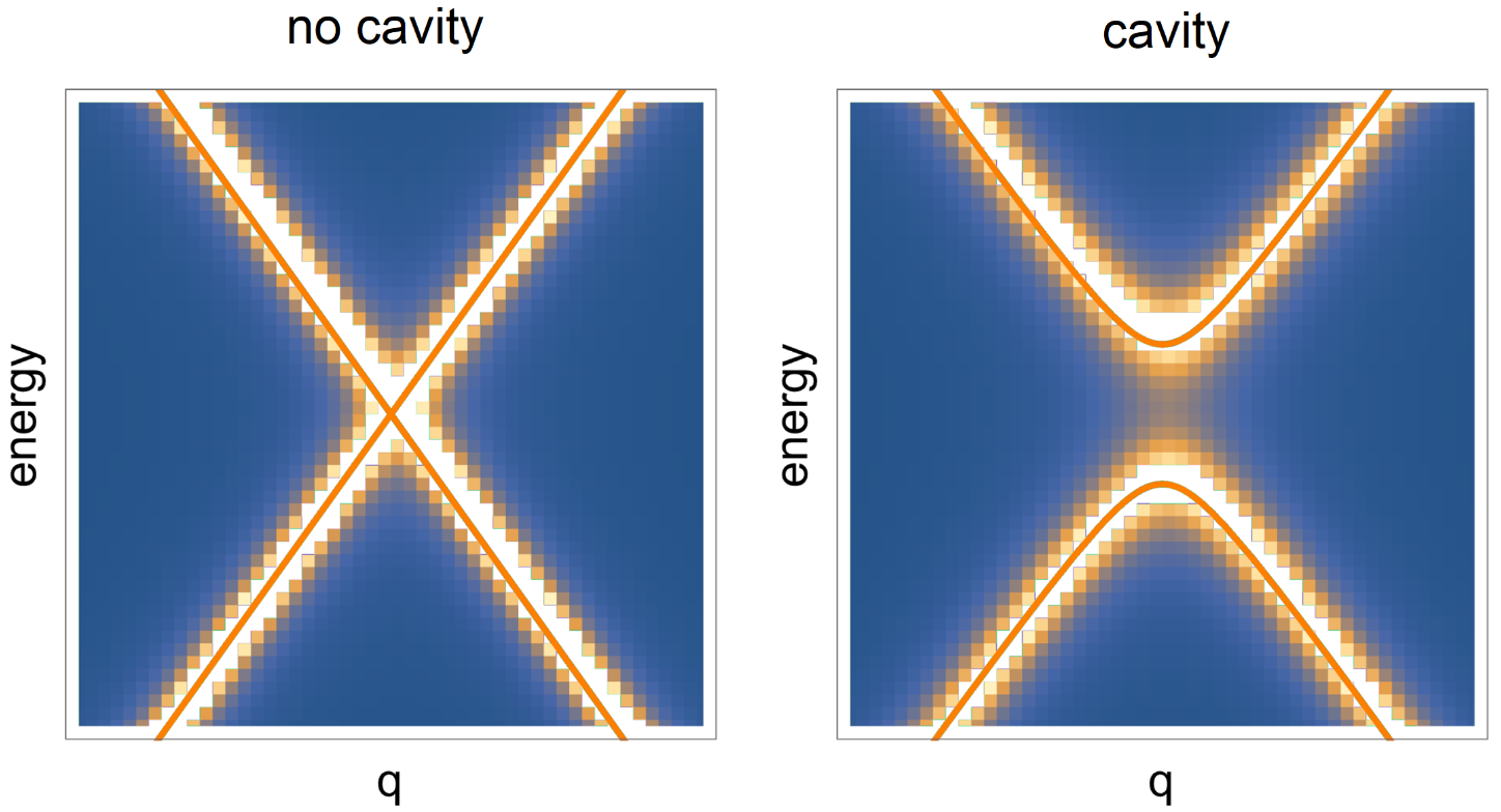
FIG. S1: The band structure near the Dirac point for monolayer graphene with time reversal symmetry (left panel) and broken time reversal symmetry (right panel). Units are arbitrary. The orange solid line is the result given by the simple theoretical model based on Eq.(S1). The color map represents the result of coupling monolayer graphene to a chiral optical cavity and computing numerically the spectral function A(ε, q) as outlined in the main text for TBG.

图 S1：具有时间反演对称性的单层石墨烯(左图)和时间反演对称性破缺的单层石墨烯(右图)在狄拉克点附近的带状结构. 单位为任意单位. 橙色实线是基于公式(S1)的简单理论模型得出的结果. 彩色图表示将单层石墨烯与手性光腔耦合并数值计算光谱函数 $A(\epsilon,\mathbf{q})$ 的结果, 如正文中针对 TBG 所概述的那样.

The role of the cavity frequency

In order to complete our analysis, we now discuss briefly the role of the characteristic frequency of the chiral optical cavity $\omega_{c}$. In the main text, we have fixed $\omega_{c} = 0.3\text{eV}$, which is a reasonable and experimentally realizable value.

In Fig.S2, we study how the electronic spectrum is modified for larger values of such a frequency. Panels (a) and (b) of Fig.S2 have to be compared with panel (d) of Fig.2 in the main text, which shows the same results for smaller $\omega_{c}$.

We observe that increasing the cavity frequency the electronic bands becomes broader and the quasi-flat bands get closer to the other gapped bands at higher energy.

Eventually, as a consequence of this strong broadening, the quasi-flat bands are not isolated anymore. This indicates that a large optical cavity frequency is detrimental in engineering isolated topological flat bands.

为了完成分析, 我们现在简要讨论一下手性光腔特征频率 $\omega_{c}$ 的作用. 在正文中, 我们固定 $\omega_{c} = 0.3\text{eV}$, 这是一个合理的、实验上可实现的值.

在图 S2 中, 我们研究了当该频率值较大时, 电子频谱是如何变化的. 图 S2 的(a)和(b)部分必须与正文中图 2 的(d)部分进行比较, 后者显示了较小 $\omega_{c}$ 时的相同结果.

我们观察到, 空腔频率 $\omega_{c}$ 越高, 电子带越宽, 能量越高时, 准平坦带越接近其他间隙带.

最终, 由于这种强烈的展宽, 准平坦带不再是孤立的. 这表明, 大的光腔频率不利于在孤立拓扑平带上进行工作.

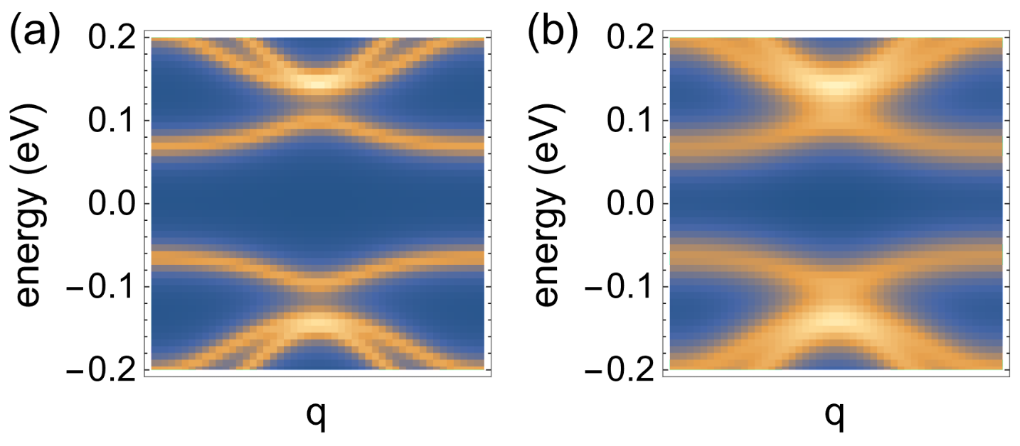
FIG. S2: The spectral function $A(\epsilon,\mathbf{q})$ showing the band structure of TBG in an optical chiral cavity for $g = 2$ and $\theta = 1.5°$. Panels (a) and (b) correspond respectively to $\omega_{c} = 0.8\text{eV}, \omega_{c} = 1.5\text{eV}$. These figures must be compared with panel (d) in Fig.2 which shows the same spectrum for $\omega_{c} = 0.3\text{eV}$.

图 S2：光谱函数 $A(\epsilon,\mathbf{q})$ 显示了光学手性腔中 TBG 在 $g = 2$ 和 $\theta = 1.5°$ 时的能带结构. 分块(a)和(b)分别对应于 $\omega_{c} = 0.8\text{eV}, \omega_{c} = 1.5\text{eV}$. 这些数字必须与图 2 中的分块 (d) 进行比较, 后者显示的是 $\omega_{c} = 0.3\text{eV}$ 时的相同光谱.

Efficiency of the cavity

In order to discuss the effect of the chiral cavity in more detail, we can define the “flattening-efficiency” as,

$$ \eta(g,\theta) = 1 - \frac{\Delta\epsilon(g,\theta)}{\Delta\epsilon(0,\theta)} $$

where $\Delta\epsilon(g,\theta)$ is the bandwidth parameter discussed in the main text. From this definition it can be found that $\eta$ takes values in the range from $0$ to $1$.

The minimum value $\eta = 0$ means that the chiral cavity has no effect on the flatness of the isolated bands.

On the contrary, the maximum value $\eta = 1$ correspond to a perfect flattening of the band after having introduce the cavity, $\Delta\epsilon(g,\theta) = 0$. More in general, a large value of $\eta$ implies that the bands are strongly flattened by the chiral cavity with respect to their structure at $g = 0$.

为了更详细地讨论手性腔的效果, 我们可以将 “平坦化效率” 定义为

$$ \eta(g,\theta) = 1 - \frac{\Delta\epsilon(g,\theta)}{\Delta\epsilon(0,\theta)} $$

其中 $\Delta\epsilon(g,\theta)$ 是正文中讨论的带宽参数. 从这个定义中可以发现, $\eta$ 的取值范围在 $0$ 到 $1$之间.

最小值 $\eta = 0$ 意味着手性腔对隔离带的平坦性没有影响.

相反, 最大值 $\eta = 1$ 对应于引入空腔后带的完全平坦化, 即 $\Delta\epsilon(g,\theta) = 0$. 更一般地说, $\eta$ 的较大值意味着, 相对于 $g = 0$ 时的结构, 手性空腔使能带被极大地扁平化.

Fig.S3 shows the flattening parameter $\eta$ as a function of the twisting angle $\theta$ and the dimensionless coupling $\widetilde{g}$ across the phase diagram, around the magic angle value $\theta = 1.1°$. We observe that, except for small $\widetilde{g}$ or near the magic angle, the chiral cavity can always greatly improve the flatness of band. The results in Fig.S3 are consistent with those reported in the main text in Fig.4.

图 S3 显示了在整个相图中, 在魔转角 $\theta=1.1°$ 附近, 平坦化参数 $\eta$ 与扭转角 $\theta$, 无量纲耦合度 $\widetilde{g}$ 的函数关系. 我们观察到, 除了较小的 $\widetilde{g}$ 和在魔幻角附近, 手性腔体总是能极大地改善波段的平坦度. 图 S3 中的结果与正文图 4 中的结果一致.

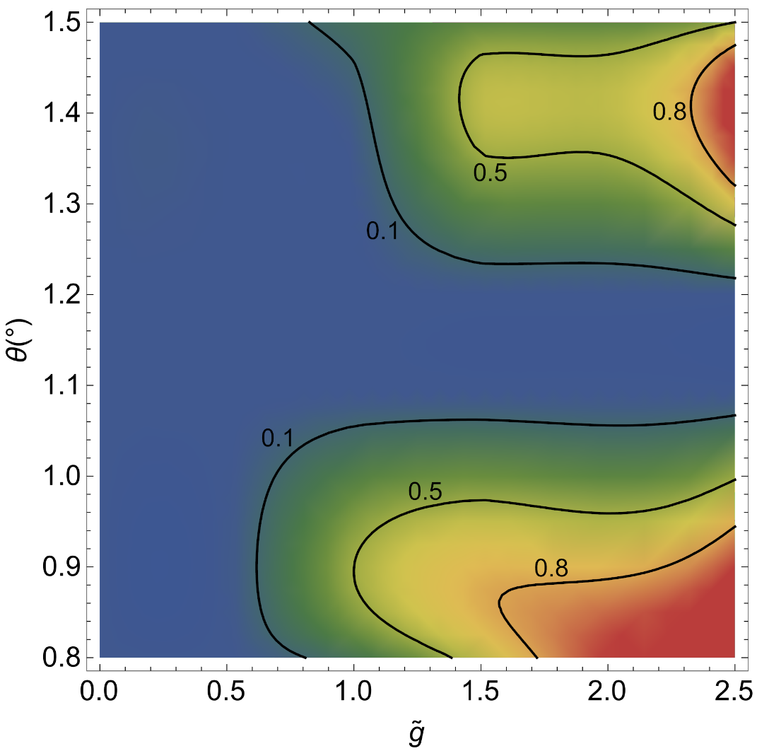
FIG. S3: The flattening efficiency parameter $\eta$ as a function of the dimensionless light-matter coupling $\widetilde{g}$ and the twisting angle $\theta$. From blue to red, the efficiency grows larger. Because the band is already flat near the magic angle, the efficiency drops to zero in there.

图 S3：平坦化效率参数 $\eta$ 与无量纲光-物质耦合参数 $\widetilde{g}$ 和扭曲角 $\theta$ 的函数关系. 从蓝色到红色, 效率越来越大. 由于能带在魔转角附近已经变平, 因此效率在该处降为 $0$.

Numerical methods and details of the setup

The Hamiltonian of monolayer graphene can be obtained by considering the hopping of electrons from one carbon atom to its three nearest neighboring atoms. The electronic band structure shows a characteristic linear dispersion relation around Fermi energy. The low energy Hamiltonian reads

$$ H_{1}(\mathbf{q}) = v_{F}\begin{pmatrix} 0 & q_{x} - iq_{y}\\ q_{x} + iq_{y} & 0 \end{pmatrix} $$

where $v_{F}$ is the Fermi velocity which is around $5.944\text{eV}\cdot Å$.

单层石墨烯的哈密顿量, 可通过考虑电子从一个碳原子跳转到其三个最近邻原子来获得. 电子能带结构在费米能级附近显示出特征的线性色散关系. 低能哈密顿量如下:

$$ H_{1}(\mathbf{q}) = v_{F}\begin{pmatrix} 0 & q_{x} - iq_{y}\\ q_{x} + iq_{y} & 0 \end{pmatrix} $$

其中, $v_{F}$ 是费米速度, 约为 $5.944\text{eV}\cdot Å$.

However, the situation in twisted bilayer graphene (TBG) is more complicated because the unit cell of the Moir ́e pattern is much larger than that of graphene. Hence, the Moir ́e Brillouin zone is quite small in reciprocal space and therefore one should consider many hopping channels between a group of Moir ́e Brillouin zones in the two layers. Below is the effective low energy Hamiltonian for TBG used in this manuscript:

$$ H_{\text{TBG}}(\mathbf{q}) = \begin{pmatrix} H_{1}(\mathbf{q}) & T_{\mathbf{q}_{b}} & T_{\mathbf{q}_{tr}} & T_{\mathbf{q}_{tl}} & \dots\\ T^{\dagger}_{\mathbf{q}_{b}} & H_{2}(\mathbf{q} - \mathbf{q}_{b}) & 0 & 0 & \dots\\ T^{\dagger}_{\mathbf{q}_{tr}} & 0 & H_{2}(\mathbf{q} - \mathbf{q}_{tr}) & 0 & \dots\\ T^{\dagger}_{\mathbf{q}_{tl}} & 0 & 0 & H_{2}(\mathbf{q} - \mathbf{q}_{tl}) & \dots\\ \vdots & \vdots & \vdots & \vdots & \ddots \end{pmatrix} $$

然而, 转角双层石墨烯(TBG)的情况更为复杂, 因为 Moir ́e 图案的单位胞比石墨烯的单位胞大得多. 因此, Moir ́e 布里渊区在倒易空间中相当小, 所以我们应该考虑两层中一组 Moir ́e 布里渊区之间的许多跃变通道. 以下是本手稿中使用的 TBG 有效低能哈密顿：

$$ H_{\text{TBG}}(\mathbf{q}) = \begin{pmatrix} H_{1}(\mathbf{q}) & T_{\mathbf{q}_{b}} & T_{\mathbf{q}_{tr}} & T_{\mathbf{q}_{tl}} & \dots\\ T^{\dagger}_{\mathbf{q}_{b}} & H_{2}(\mathbf{q} - \mathbf{q}_{b}) & 0 & 0 & \dots\\ T^{\dagger}_{\mathbf{q}_{tr}} & 0 & H_{2}(\mathbf{q} - \mathbf{q}_{tr}) & 0 & \dots\\ T^{\dagger}_{\mathbf{q}_{tl}} & 0 & 0 & H_{2}(\mathbf{q} - \mathbf{q}_{tl}) & \dots\\ \vdots & \vdots & \vdots & \vdots & \ddots \end{pmatrix} $$

In this effective Hamiltonian, $H_{1,2}$ indicate the Hamiltonian of the top/bottom layer. Moreover, $\mathbf{q}_{b} = \frac{1}{3}(\mathbf{b}_{1}^{m} - \mathbf{b}_{2}^{m}), \mathbf{q}_{tr} = \frac{1}{3}(\mathbf{b}_{1} + 2\mathbf{b}_{2}^{m}),\mathbf{q}_{tl} = \frac{1}{3}(-2\mathbf{b}_{1}^{m}-\mathbf{b}_{2}^{m})$, where $\mathbf{b}_{1}^{m}$ and $\mathbf{b}_{2}^{m}$ are Moir`e reciprocal vectors. The twisting angle $\theta$ is hidden in these vectors. The hopping matrix elements are given by,

$$ T_{\mathbf{q}_{b}} = t\left(\begin{array}{cc} 1 & 1 \\ 1 & 1 \end{array}\right),\quad T_{\mathbf{q}_{tr}} = t\left(\begin{array}{cc} e^{i\phi} & 1 \\ e^{-i\phi} & e^{i\phi} \end{array}\right),\quad T_{\mathbf{q}_{tl}} = t\left(\begin{array}{cc} e^{-i\phi} & 1 \\ e^{i\phi} & e^{-i\phi} \end{array}\right) $$

where $\phi = \frac{2\pi}{3}$ and $t = 0.11$ is the hopping parameter.

在这个有效哈密顿中, $H_{1,2}$ 表示顶层/底层的哈密顿量. 此外, $\mathbf{q}_{b} = \frac{1}{3}(\mathbf{b}_{1}^{m} - \mathbf{b}_{2}^{m}), \mathbf{q}_{tr} = \frac{1}{3}(\mathbf{b}_{1} + 2\mathbf{b}_{2}^{m})、\mathbf{q}_{tl} = \frac{1}{3}(-2\mathbf{b}_{1}^{m}-\mathbf{b}_{2}^{m})$ , 其中 $\mathbf{b}_{1}^{m}$ 和 $\mathbf{b}_{2}^{m}$ 是 Moir`e 的倒易矢量. 扭曲角 $\theta$ 隐藏在这些向量中. 跳跃矩阵元由以下公式给出：

$$ T_{\mathbf{q}_{b}} = t\left(\begin{array}{cc} 1 & 1 \\ 1 & 1 \end{array}\right),\quad T_{\mathbf{q}_{tr}} = t\left(\begin{array}{cc} e^{i\phi} & 1 \\ e^{-i\phi} & e^{i\phi} \end{array}\right),\quad T_{\mathbf{q}_{tl}} = t\left(\begin{array}{cc} e^{-i\phi} & 1 \\ e^{i\phi} & e^{-i\phi} \end{array}\right) $$

其中, $\phi = 2\pi/3$ 和 $t = 0.11$ 是跃变参数.

It should be noticed here that the Hamiltonian matrix of TBG shown in Eq.(S5) is not of dimension 8 × 8. Indeed, one should extend the matrix Eq.(S5) by taking into account more bases to obtain the flat band at the magic angle.

For example, in the basis $|l,(m,n)\rangle, l = 1,2$ indicates the top/bottom layer, while $m,n = -2,-1,0,1,2$ indicates the combination of two Moire reciprocal vectors, namely $\langle l,(m,n)|l,(m,n)\rangle = H_{l}(\mathbf{q} + (l - 1)\mathbf{q}_{b} + m\mathbf{b}_{1}^{m} + n\mathbf{b}_{2}^{m})$. According to this formula, the Hamiltonian matrix should be $100\times 100$ dimensional.

这里需要注意的是, 公式(S5)中所示的 TBG 的哈密顿矩阵并不是 8 × 8 维的. 事实上, 我们应该通过考虑更多的基数来扩展公式(S5)矩阵, 以获得魔幻角处的平带.

例如, 在基矢 $|l,(m,n)\rangle 中, l = 1,2$ 表示顶层/底层, 而 $m,n = -2,-1,0,1,2$ 表示两个摩尔倒易矢量的组合, 即 $\langle l,(m,n)|l,(m,n)\rangle = H_{l}(\mathbf{q} + (l - 1)\mathbf{q}_{b} + m\mathbf{b}_{1}^{m} + n\mathbf{b}_{2}^{m})$. 根据这个规则, 哈密顿矩阵应该是 $100\times 100$ 维的.

As outlined in the main text, in principle the self-energy is given by an infinite sum over the Matsubara frequencies as

$$ \Sigma_{0}(\epsilon,\mathbf{q}) = -\frac{g^{2}}{\beta}\sum_{m = 1}^{\infty}G_{0}(\epsilon + i\omega_{m},\mathbf{q})D_{0}(\omega_{m}) $$

where $\omega_{m} = 2\pi mk_{B}T$ is the Matsubara frequency and $g$ the coupling parameter between photon and electron.

如正文所述, 原则上, 自能是由松原频率的无限级数和给出的, 即

$$ \Sigma_{0}(\epsilon,\mathbf{q}) = -\frac{g^{2}}{\beta}\sum_{m = 1}^{\infty}G_{0}(\epsilon + i\omega_{m},\mathbf{q})D_{0}(\omega_{m}) $$

其中, $\omega_{m} = 2\pi mk_{B}T$ 是松原频率, $g$ 是光子和电子之间的耦合参数.

Nevertheless, from a computational perspective, the Matsubara frequency summation in Eq.(S7) is performed by introducing a finite UV cutoff $N$

$$ \Sigma_{0}(\epsilon,\mathbf{q}) = -\frac{g^{2}}{\beta}\sum_{m = 1}^{N}G_{0}(\epsilon + i\omega_{m},\mathbf{q})D_{0}(\omega_{m}) $$

The computations shown in the main text are for $N = 100$. To make sure that the sum converged for the value of the cutoff used in the main text, we have computed the same spectral function with different cutoffs as shown in Fig.S4. The results show only little difference upon changing the cutoff from $N = 50$ to $N = 150$ confirming that the numerical method is reliable.

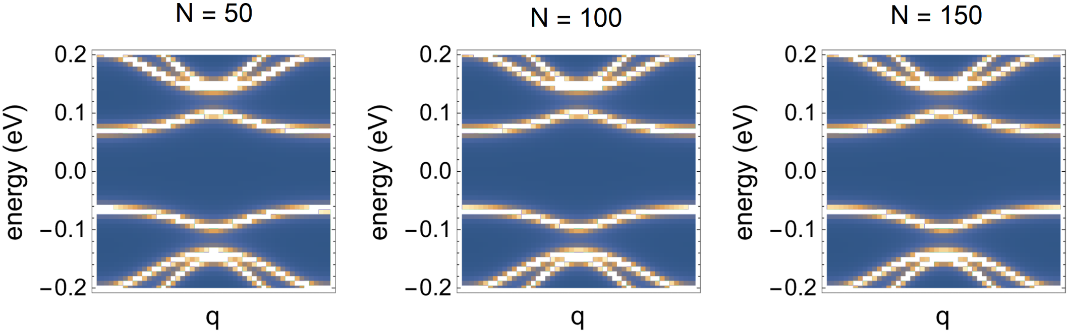
S4: The results for the self-energy Eq.(S8) using different values of the cutoff. From left to right, $N = 50,N = 100, N = 150$ while $\theta = 1.5°, g = 2$. This figure emphasizes the stability of our numerical routine and its convergence as a function of the cutoff $N$.

S4: 使用不同截止值计算自能方程(S8)的结果. 从左到右, $N = 50, N = 100, N = 150$, 而 $\theta = 1.5°, g = 2$. 该图强调了我们的数值计算程序的稳定性及其收敛性与截止值 $N$ 的函数关系.

Finally, let us emphasize that the propagator used in the main text is just the lowest order self-energy without any self consistent calculation. To obtain more accurate results, one should obtain the two solutions, $G[\Sigma]$ and $\Sigma[G]$, consistently by iteration algorithm. However, the lowest order self energy is enough to grasp the main features.

最后, 我们要强调的是, 正文中使用的传播子只是最低阶自能, 没有任何自洽性计算. 为了得到更精确的结果, 我们应该通过迭代算法得到 $G[\Sigma]$ 和 $\Sigma[G]$ 这两个一致的解. 然而, 最低阶自能足以把握主要特征.