Abstract
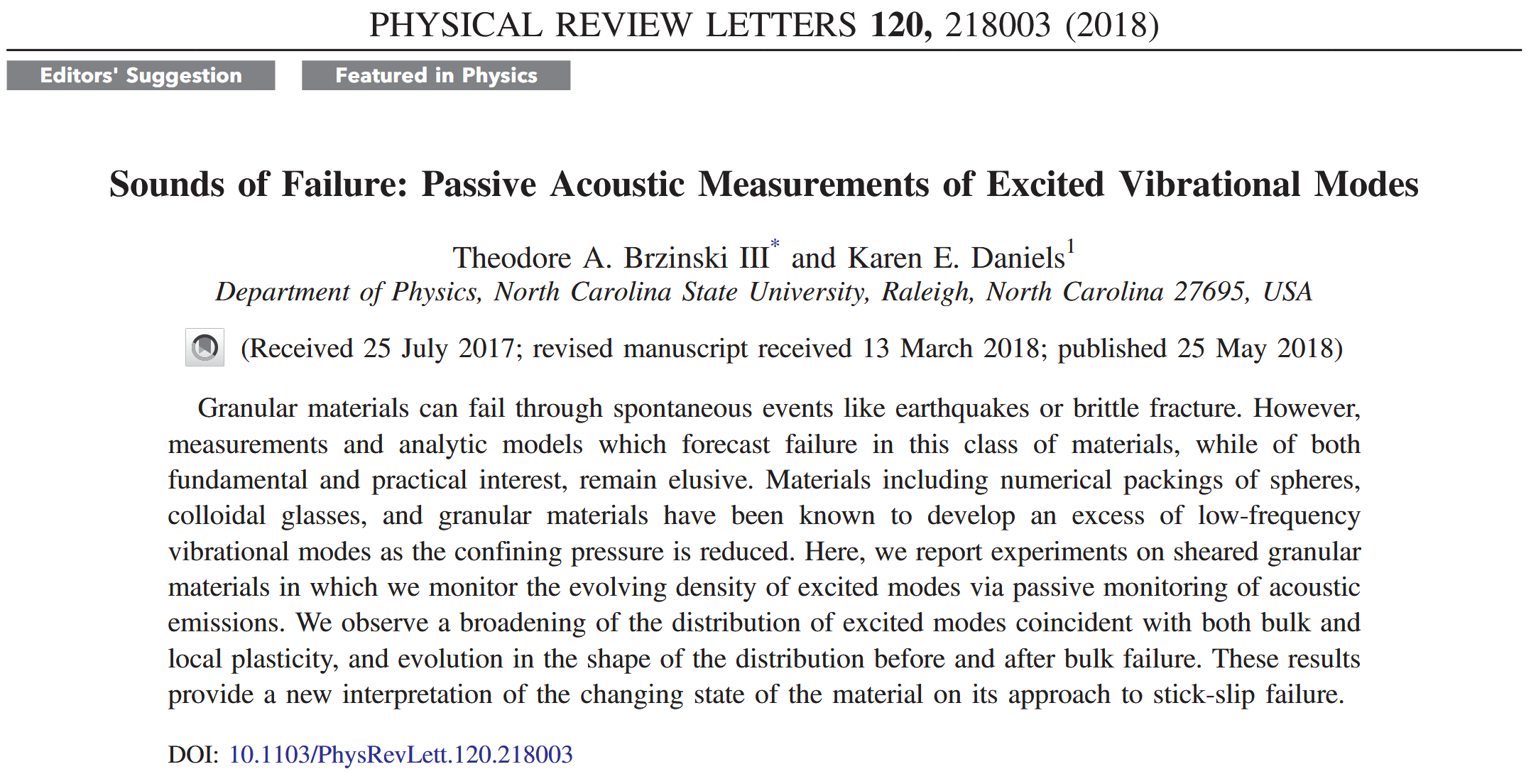
Granular materials can fail through spontaneous events like earthquakes or brittle fracture. However, measurements and analytic models which forecast failure in this class of materials, while of both fundamental and practical interest, remain elusive. Materials including numerical packings of spheres, colloidal glasses, and granular materials have been known to develop an excess of low-frequency vibrational modes as the confining pressure is reduced.
颗粒材料会因地震或脆性断裂等自发事件而破坏。然而,能够预测这类材料破坏的测量结果和分析模型,虽然具有基础性和实用性,但仍然难以捉摸。众所周知,包括球体的数值堆积、胶体玻璃和颗粒材料在内的材料会随着约束压力的降低而产生过多的低频振动模式。
Here, we report experiments on sheared granular materials in which we monitor the evolving density of excited modes via passive monitoring of acoustic emissions. We observe a broadening of the distribution of excited modes coincident with both bulk and local plasticity, and evolution in the shape of the distribution before and after bulk failure. These results provide a new interpretation of the changing state of the material on its approach to stick-slip failure.
在这里,我们报告了在剪切颗粒材料上进行的实验,在这些实验中,我们通过 被动监测 声发射来监控激发模式密度的演变。我们观察到激发模式分布的扩大与整体塑性和局部塑性相吻合,以及整体破坏前后分布形状的演变。这些结果为材料在接近滞滑破坏时的状态变化提供了新的解释。
Introduction
The framework provided by the jamming transition has highlighted the extent to which granular and other amorphous systems share certain properties: spatially and dynamically heterogeneous response to stress, structural disorder, and inhomogeneous force transmission.
While the onset of rigidity in jammed materials shares features with standard second-order phase transitions, jamming differs from other such transitions by its lack of a diverging structural length scale.
堵塞转变所提供的框架凸显了颗粒和其他非晶态系统在多大程度上具有某些共同特性:对 应力 的空间和动态异质响应、结构紊乱和非均匀力传输。
虽然堵塞材料的刚性开始与标准二阶相变具有相同的特征,但堵塞与其他此类转变的不同之处在于它缺乏发散的结构长度尺度。
Although jammed systems are not necessarily thermal, it has been observed that the density of vibrational modes $D(\omega)$ remains an important descriptor of the state of the system.
In particular, an excess of low-frequency modes develops on the approach to the jamming transition and the onset of plasticity. Indeed, these excess low-frequency modes have been observed in experiments in colloidal systems as well as granular materials.
虽然堵塞系统并不一定是热系统,但据观察,振动模式密度 $D(\omega)$ 仍然是系统状态的重要描述指标。
特别是,在接近堵塞转变和塑性开始时,会出现低频模态过剩的现象。事实上,在胶体系统和颗粒材料的实验中都观察到了这些过剩的低频模态。
As such, both experiments and simulations tantalizingly suggest that information about the rigidity of a system might be encoded within $D(\omega; t)$ as the system evolves under external loading (thus, the notation to denote its values at a specific time $t$). $D(\omega;t)$ is a particularly attractive metric since the passive recording of acoustic emissions provides a noninvasive method of reporting changes in the state of the system and does not require visual access to the system.
因此,实验和模拟都诱人地表明,当系统在外部负载下演变时,系统刚度的信息可能被编码在 $D(\omega;t)$ 中(因此,用符号表示其在特定时间 $t$ 的值)。$D(\omega;t)$ 是一个特别有吸引力的指标,因为被动记录声发射提供了一种报告系统状态变化的非侵入式方法,而且不需要对系统进行可视访问。
For example, embedded sensors have long been used for nondestructive evaluation of engineered structures, and have also successfully identified precursors in volcanic systems.
例如,嵌入式传感器长期以来一直用于工程结构的无损评估,并成功识别了火山系统中的前兆。
One practical method for measuring $D(\omega;t)$ has been to take advantage of the relationship between the particle velocity autocorrelation function and the density of vibrational modes. Recent experiments on a quasi-2D granular packing have used this relationship to establish a connection between acoustic modes and the jamming framework. The procedure is to measure the velocity autocorrelation function
$$ C_{v}(t)\equiv \frac{\sum v_{k}(t+\tau)v_{k}(t)}{\sum v_{k}(t)v_{k}(t)}.\tag{1}\label{eq1} $$
which is a function of both time $(t)$ and lag time $(\tau)$. Here, $v_{k}(\tau)$ is the velocity time series measured using the $k$th of many particle-scale piezoelectric sensors; the sums over $k$ cover all sensors in the system. The density of vibrational modes is then given by
$$ D(\omega; t) = \int_{0}^{+\infty} C_{v}(\tau;t)\cos{(2\pi\omega\tau)}\mathrm{d}\tau. \tag{2}\label{eq2} $$
测量 $D(\omega;t)$ 的一种实用方法是利用 颗粒速度自动关联函数 与振动模式密度之间的关系。最近对准二维颗粒堆积进行的实验利用这种关系建立了声学模式与堵塞框架之间的联系。其步骤是测量速度自相关函数
$$ C_{v}(t)\equiv \frac{\sum v_{k}(t+\tau)v_{k}(t)}{\sum v_{k}(t)v_{k}(t)}.\tag{1} $$
是时间 $(t)$ 和滞后时间 $(\tau)$ 的函数。这里,$v_{k}(\tau)$ 是使用众多颗粒尺度级别的压电传感器中的第 $k$ 所测得的速度时间序列;对 $k$ 的求和涵盖了系统中的所有传感器。振动模式的密度为
$$ D(\omega; t) = \int_{0}^{+\infty} C_{v}(\tau;t)\cos{(2\pi\omega\tau)}\mathrm{d}\tau. \tag{2} $$
This approach succeeds even for measurements over a small subset of the particles, recovering the expected Debye scaling for crystalline granular materials as well as the expected excess of low-$\omega$ modes in both amorphous and crystalline systems as the confining pressure was reduced.
即使是对一小部分颗粒进行测量,这种方法也能取得成功。随着约束压力的降低,结晶的颗粒材料恢复了预期的 Debye 幂律比例,无定形和晶体系统中的低 $\omega$ 模式也恢复了预期的过量。
Our experiments are inspired by prior work on slowly loaded granular materials, from which it is known that (1) particle-scale rearrangements both precede and follow failure events, and (2) acoustic emissions and microslips show an exponential increase in their rate of occurrence leading up to a failure event and have been shown to encode information about the internal strength of the material.
Here, we measure the acoustic emissions during the lead up to failure, and associate changes in the observed $D(\omega, t)$ with the approach to failure. In doing so, we provide a new means of acoustic monitoring.
我们的实验受到之前关于缓慢加载颗粒材料的工作的启发,从这些工作中我们知道:(1) 颗粒尺度的重排既发生在失效事件之前,也发生在失效事件之后;(2) 声发射和微滑动在失效事件之前的发生率呈指数增长,并已被证明编码了材料内部强度的信息。
在此,我们测量了失效前的声发射,并将观测到的 $D(\omega, t)$ 的变化与失效的临近联系起来。这样,我们就提供了一种新的声学监测手段。
Unlike spectral power measurements, which capture the distribution of acoustic power among modes of different frequencies, the approach we introduce is effectively a measurement of the number of modes which are excited, regardless of the excitation amplitude. To differentiate from the actual density of vibrational modes, we denote this measurement as the density of excited modes, $D_{\text{ex}}(f;t)$, where $f$ replaces $\omega$ as frequency. As far as we know, there are no theoretical expectations for the behavior of $D_{\text{ex}}$; what follows is an empirical exploration.
频谱功率测量捕捉的是不同频率模态之间的声功率分布,与此不同,我们引入的方法实际上是测量被激发的模态数量,与激发振幅无关。为了区别于实际的振动模式密度,我们将这种测量方法称为受激模密度,即 $D_{\text{ex}}(f;t)$,其中 $f$ 代替 $\omega$ 作为频率。据我们所知,$D_{\text{ex}}$ 的行为不存在理论预期;下面将进行经验性探索。
Experimental Methods
Our experiment, depicted in Figs. 1(a)–1(c), comprises an annulus with an outer wall of diameter $66.75\text{ cm}$ and an inner wall of diameter $30.5\text{ cm}$. The system is filled with a single layer of approximately $8000$ grains. The grains are a $60∶40$ mixture of $5.6\text{ mm}$ circular and $4.9$ by $6.9\text{ mm}$ elliptical disks to prevent crystallization. All grains are milled from PhotoStress Plus PS-3 polymer from the Vishay Measurements Group with a bulk elastic modulus of $0.21\text{ GPa}$.
我们的实验如图 1(a)-1(c) 所示,包括一个外壁直径为 $66.75\text{ cm}$ ,内壁直径为 $30.5\text{ cm}$ 的环形结构。该系统由约 $8000$ 个颗粒组成的单层填充。为防止结晶,这些颗粒是由 $5.6\text{ mm}$ 球形和 $4.9\times 6.9\text{ mm}$ 椭圆形 $60:40$ 的混合物。所有颗粒均由 Vishay Measurements Group 的 PhotoStress Plus PS-3 聚合物研磨而成,其体积弹性模量为 $0.21\text{ GPa}$。
The granular material is sheared at a rate of one rotation per hour via a torsion spring [pictured in Fig. 1(b)] with a stiffness of $0.85\text{ N m/rad}$ and maximum compression of $26^{\circ}$, corresponding to a torque of $0.39\text{ N m}$. Twelve (12) piezoelectric sensors, which are embedded in the outer wall, produce a voltage proportional to any compressive force they experience, thus registering a measurement of the acoustic emissions of the granular material. During an experiment, the driving torque [Fig. 1(d)] and acoustic emissions [(Fig. 1(e))] of the system are continuously measured via a torque sensor (Cooper Instruments) and acoustic sensors (detailed in [20]).
颗粒材料通过扭转弹簧(如图 1(b) 所示)以每小时旋转一圈的速度进行剪切,扭转弹簧的刚度为 $0.85\text{ N m/rad}$,最大压缩量为 $26^{\circ}$ ,对应扭矩为 $0.39\text{ N m}$。嵌入外壁的十二(12)个压电传感器会产生与其所受压缩力成正比的电压,从而记录颗粒材料声发射的测量值。在实验过程中,系统的驱动扭矩 [图 1(d)] 和声发射 [图 1(e)] 通过扭矩传感器(Cooper Instruments 公司)和声传感器(详见 [20])进行连续测量。
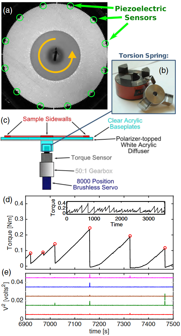
(a) Top view of the annular shear cell, with piezoelectric sensors and moving (inner) wall. (b) Drive shaft coupling with Hookean torsion spring. (c) Schematic side view illustrating the details of the drive system. (d) Sample torque data over the course of ten minutes and (inset) one hour. Red circles identify slips. (e) Sample measurements of the voltage squared, $V^{2}(t)$, measured for five piezoelectric sensors, vertically offset and plotted on the same time axis as (d).
(a) 带有压电传感器和可动(内)壁的环形剪切单元俯视图。(b) 带胡克式扭转弹簧的传动轴联轴器。(c) 驱动系统细节示意侧视图。(d) $10$ 分钟和(插图)$1$ 小时的扭矩数据样本。红圈表示滑动。(e) 五个压电传感器的电压平方 $V^{2}(t)$,垂直偏移并绘制在与 (d) 相同的时间轴上。
This driving produces intermittent stick-slip failure events, apparent as the sawtooth features in Fig. 1(d). The loading (stick) phase corresponds to the compression of the torsional spring, and when the applied torque surpasses the strength of the granular material, failure (slip) occurs. Empirically, after an initial transient, the frequency of slips remains close to $1\text{ slip/minute}$.
这种驱动会产生间歇性的粘滞-滑移失效事件,如图 1(d)中的锯齿特征所示。加载(粘连)阶段对应于扭转弹簧的压缩,当施加的扭矩超过颗粒材料的强度时,就会发生破坏(滑移)。根据经验,在初始瞬态之后,滑移的频率会保持在 $1$ 滑移/分钟。
The data presented here were all collected in this steady state over the course of $23$ hours. The full dataset of $1165$ slip events are aperiodic and span a broad range of torque and time scales [see the inset in Fig. 1(d)], indicating substantial heterogeneity in the material strength and degree of deformation.
本文所展示的数据都是在 $23$ 小时的稳定状态下收集的。$1165$ 滑移事件的完整数据集是非周期性的,并且涵盖了广泛的扭矩和时间尺度范围[见图 1(d) 的插图],这表明材料强度和变形程度存在很大的异质性。
Despite the spatiotemporal heterogeneity, the slip durations exhibit a relatively narrow distribution with a mean of $0.65\pm 0.14\text{ s}$. This slipping timescale is well-separated from the interslip (quiescent) timescale: more than $80\%$ of slips, are preceded and followed by quiescent periods of $30$ seconds or more. We focus our analysis on the subset of these $887$ slips to isolate the effects of individual events.
尽管存在时空异质性,但滑动持续时间呈现出相对狭窄的分布,平均值为 $0.65\pm 0.14\text{ s}$。这种滑动时间尺度与滑动间(静止)时间尺度有很好的分隔:超过 $80\%$ 的滑动前后都有 $30$ 秒或更长的静止期。我们把分析重点放在这些 $887$ 个滑动子集上,以分离出单个事件的影响。
An illustration of the typical intermittency of the acoustic emissions is provided in Fig. 1(e); each trace is the power from one piezoelectric sensor. We observe that the largest emissions always coincide with slips. Importantly, the converse is not the case: not every slip produces a voltage spike in every sensor. This behavior arises because the force chains cause spatial heterogeneities in acoustic transmission.
图 1(e) 显示了声发射的典型间歇性;每个轨迹都是来自一个压电传感器的功率。我们观察到,最大的声发射总是与滑动同时发生。重要的是,情况并非如此:并非每次滑动都会在每个传感器中产生电压尖峰。产生这种现象的原因是力链导致了声波传播的空间异质性。
The typical rms voltage during quiescent periods (without large torque drops) is $2.0\text{ mV}$, the noise floor of our data acquisition hardware is $1.34\text{ mV}$, and emission events can produce spikes as much as $3$ orders of magnitude higher. In this Letter, we investigate the lowamplitude emissions during the largely quiescent periods between these slips.
静态期间(无大扭矩下降)的典型均方根电压为 $2.0\text{ mV}$,我们的数据采集硬件的本底噪声为 $1.34\text{ mV}$,而发射事件可产生高出 $3$ 个数量级的尖峰。在这封信中,我们研究了在这些滑动之间的基本静止期间的低振幅发射。
We analyze the evolution of the density of excited states, $D_{\text{ex}}(f;t-t_{i})$, by the following procedure: for each sensor and slip event occurring at time $t_{i}$, we divide the voltage time series into $61 1\text{ s}$ intervals centered around $t_{i}$; we integrate the voltage over each interval to obtain the sensor velocities in arbitrary units; we calculate $D_{\text{ex}}(f)$ via Eqs. (1) and (2) (see Supplemental Material); we plot this quantity as a function of frequency ($f$) and ($t − t_{i}$) in modograms. Sample modograms for four events are shown in Fig. 2(b). One prominent feature is that a broad range of modes is excited during each slip ($t = t_{i}$).
我们通过以下步骤分析激发态密度($D_{\text{ex}}(f;t-t_{i})$)的演变:对于每个传感器和发生在 $t_{i}$ 时间的滑移事件,我们将电压时间序列划分为以 $t_{i}$ 为中心的 $61$ 个 $1\text{ s}$ 区间;我们对每个区间的电压进行积分,以获得以任意单位 (a.u.) 表示的传感器速度;我们通过公式 (1) 和 (2) 计算 $D_{\text{ex}}(f)$(见补充材料);我们用模态图绘制该量与频率($f$)和($t - t_{i}$)的函数关系。(1) 和 (2) 计算出 $D_{\text{ex}}(f)$(见补充材料);我们将此量绘制成频率 ($f$) 和 ($t - t_{i}$) 的函数模态图。四个事件的模态图样本见图 2(b)。一个显著特点是,在每次滑移($t = t_{i}$)过程中,都会激发出多种模式。
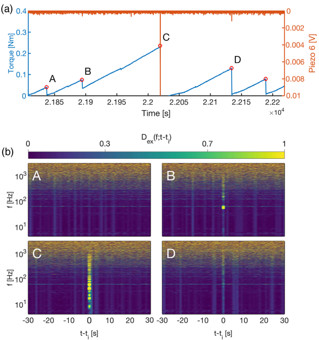
(a) $400\text{ s}$ of torque (blue) and voltage (red) measurements from one piezoelectric sensor. Five slips are labeled with red circles. (b) Sample modograms showing the density of excited modes $D_{\text{ex}}(f;t-t_{i})$ for an interval of $\pm 30\text{ s}$ centered on each of the four labeled slips (A)–(D).
(a) 一个压电传感器测量的扭矩(蓝色)和电压(红色)的 $400\text{ s}$。红色圆圈标注了五个滑动点。(b) 模态图样本,显示以四个标注滑块(A)-(D)为中心的 $\pm 30\text{ s}$ 间隔内的激发模态密度 $D_{\text{ex}}(f;t-t_{i})$。
However, similar increases in excited modes are also observed at times before and after the slips; these features are visible as bright vertical bands in Fig. 2(b). We also observe that the overall density of excited modes appears to be relatively flat over nearly three decades (Hz to kHz), rising only at the highest frequencies in this range. Finally, we observe several persistent frequencies which appear as horizontal lines. While the $60\text{ Hz}$ peak is of electronic origin, the others are likely due to acoustic noise such as from the drive system or building noise. These noise peaks will be filtered out in the later stages of analysis.
不过,在滑移前后也观察到激发模式的类似增加;这些特征在图 2(b)中以明显的垂直带的形式显示出来。我们还观察到,在近 $3$ 个数量级($\text{ Hz}$ 到 $\text{ kHz}$)的范围里,激发模式的总体密度似乎相对平缓,只有在这一范围内的最高频率才会上升。最后,我们观察到几个持续存在的频率,它们以水平线的形式出现。虽然 $60\text{ Hz}$ 的峰值是由电子引起的,但其他峰值很可能是由声学噪声引起的,如来自驱动系统或建筑物的噪声。这些噪音峰值将在后期分析阶段被过滤掉。
We begin by focusing on the vertical bands visible in Fig. 2(b). Each of these bands represents a time at which a single piezoelectric sensor detected an increase in the number of excited vibrational modes over a broad range of frequencies. Some of these vertical bands correspond to global slip events ($t = t_{i}$), but most are detected due to local rearrangements which happened to occur close to a particular sensor. The local nature of these detections is reinforced by the observation that modograms from different sensors do not all record increases [as also seen in Fig. 1(e)].
我们首先关注图 2(b) 中可见的垂直条带。这些条带中的每一条都代表了单个压电传感器检测到激发振动模式数量在广泛频率范围内增加的时间。这些垂直条带中的一些与全局滑移事件($t = t_{i}$)相对应,但大多数是由于靠近特定传感器的局部重排而检测到的。来自不同传感器的模态图并不都记录有增加[如图 1(e)所示],这一观察结果加强了这些检测的 局域性。
The ability to measure the $D_{\text{ex}}(f;t-t_{i})$ from either low- or high-amplitude slip events is crucially important to this method. While the low-amplitude events are too small to cause a global slip event, some of them are, nonetheless, large enough to be detected as they travel through the granular material and, thereby, leave a record of the state of the material. As we shall see below, the information they transmit reveals the changing state of the material.
测量来自低振幅或高振幅滑移事件的 $D_{\text{ex}}(f;t-t_{i})$ 的能力对该方法至关重要。虽然低振幅事件太小,无法引起整体滑移事件,但其中一些事件的规模足够大,可以在穿过颗粒材料时被检测到,从而留下材料状态的记录。我们将在下文中看到,它们传递的信息揭示了材料状态的变化。
In order to reduce the impact of noise in the density of excited modes, we construct the average modogram $\tilde{D}_{\text{ex}}(f;t-t_{i})\equiv \langle D_{\text{ex}}(f;t-t_{i})\rangle_{i,k}$, where $i$ is an index over the $887$ detected slips separated by at least $30\text{ s}$ from the adjacent slips, and $k$ is an index over the $12$ sensors.
为了减少激发模式密度中噪声的影响,我们构建了平均模态图 $\tilde{D}_{\text{ex}}(f;t-t_{i})\equiv \langle D_{\text{ex}}(f;t-t_{i})\rangle_{i,k}$ ,其中 $i$ 是 $887$ 检测到的滑动点的索引,与相邻滑动点的距离至少为 $30\text{s}$,$k$ 是 $12$ 个传感器的索引。
To highlight the relative changes this quantity exhibits in response to failure and to suppress persistent electronic or physical resonances, we normalize $\tilde{D}_{\text{ex}}$ by the sensor- and time-averaged density of excited states, $B(f) = \langle\tilde{D}_{\text{ex}}(f;t-t_{i})\rangle_{t\neq t_{i}}$ to obtain the rescaled modogram shown in Fig. 3.
为了突出这个量在响应破坏时的相对变化,并抑制持续的电子或物理共振,我们将 $\tilde{D}_{\text{ex}}$ 归一化为传感器和时间平均的激发态密度,即 $B(f) = \langle\tilde{D}_{\text{ex}}(f;t-t_{i})\rangle_{t\neq t_{i}}$ ,从而得到图 3 所示的重标度模态图。
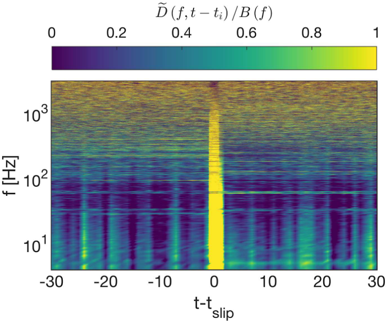
Average modograms $\tilde{D}_{\text{ex}}(f;t-t_{i})$, taken over $887$ slips and $12$ sensors and normalized by the sensor- and time-averaged density of excited states, $B(f)$.
平均模态图 $\tilde{D}_{\text{ex}}(f;t-t_{i})$,数据来自 $887$ 个滑动和 $12$ 个传感器,并以传感器和时间平均激发态密度 $B(f)$ 归一化。
This normalized average modogram exhibits features similar to the fluctuations observed in Fig. 2, but now, the vertical streaks result from the average behavior over many slips and sensors.
The remaining heterogeneity indicates that $887$ slips were an insufficient quantity of data to eliminate the temporal heterogeneity associated with localized plasticity. Even within this noisy signal, however, there emerge clear differences between the preslip and postslip portions of this modogram.
这个归一化平均模态图显示出与图 2 中观察到的波动相似的特征,但现在,垂直条纹是由许多滑动和传感器的平均行为产生的。
剩余的异质性表明,$887$ 个滑动的数据量不足以消除与局部可塑性相关的时间异质性。不过,即使在这种噪声信号中,该模态图的滑动前和滑动后部分也存在明显差异。
To characterize the changes in the slip- and sensor-averaged $\tilde{D}_{\text{ex}}$, we calculate the first four moments of that quantity. These are best considered as empirical shape parameters, since there is no prediction for the shape of $\tilde{D}_{\text{ex}}$, and our dynamic range may capture only a portion of the distribution. Nonetheless, a clear signal is evident in these quantities (Fig. 4).
We find that the mean frequency (a) gradually grows during the preslip phase, and then, suddenly decreases from $1.60$ to $1.59\text{ kHz}$ (less than $1\%$) in response to slips.
为了描述滑移和传感器平均值 $\tilde{D}_{\text{ex}}$ 的变化特征,我们计算了该量的前四个矩。这些最好被视为经验形状参数,因为我们无法预测 $\tilde{D}_{\text{ex}}$ 的形状,而且我们的动态范围可能只能捕捉到分布的一部分。尽管如此,这些量中还是有明显的信号(图 4)。
我们发现,平均频率(a)在滑动前阶段逐渐增长,然后在滑动时突然从 $1.60$ 下降到 $1.59\text{ kHz}$(小于 $1\%$)。
This effect is accompanied by a small increase in the variance (b) If our dynamic range captures most of the excited modes, these changes are consistent with a broadening of $\tilde{D}_{\text{ex}}(f)$ in response to failure, with excited modes arising at lower-frequencies.
Since the internal stress in the granular material is lower after a slip [see Fig. 1(d)], these observations are consistent with the observations of failure of the force chain network and emergence of excess low-frequency modes at smaller confining stresses.
如果我们的动态范围捕捉到了大部分激发模式,那么这些变化与 $\tilde{D}_{\text{ex}}(f)$ 在响应失效时的拓宽一致,激发模式出现在较低频率上。
由于滑移后颗粒材料的内应力降低[见图 1(d)],这些观察结果与力链网络失效以及在较小约束应力下出现过量低频模态的观察结果是一致的。
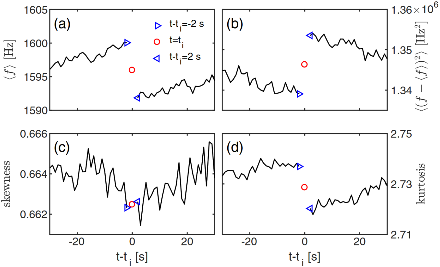
The four moments of $\tilde{D}_{\text{ex}}(f;t-t_{i})$, calculated at fixed times preslip and postslip: (a) mean frequency, (b) variance, (c) skewness, and (d) kurtosis. The red “circles” indicates the time of the slip (data point omitted for clarity). The right- and left-pointing cyan triangles indicate the values immediately before and after the slip.
在滑动前和滑动后固定时间计算的 $\tilde{D}_{\text{ex}}(f;t-t_{i})$ 的四个矩:(a) 平均频率,(b) 方差,(c) 偏度,(d) 峰度。红色 “圆圈” 表示滑动时间(为清晰起见省略数据点)。右侧和左侧的青色三角形表示滑移前后的数值。
We also observe similarly clear, but still small, signals in the higher central moments of $\tilde{D}_{\text{ex}}$: a weak minimum in skewness and a $1\%$ drop in the kurtosis [panels (c)–(d), respectively]. We find a skewness of $0.66$, which means low-frequency modes are more common than high-fre- quency modes. The kurtosis close to $3$ indicates $\tilde{D}_{\text{ex}}$ is neither particularly heavy nor weak tailed.
在 $\tilde{D}_{\text{ex}}$ 的较高中心矩中,我们也观察到了类似明显但仍然微小的信号:偏度出现微弱的最小值,峰度下降了 $1\%$ [分别为子图 (c)-(d)]。我们发现偏度为 $0.66$,这意味着低频模式比高频模式更为常见。接近 $3$ 的峰度表明,$\tilde{D}_{\text{ex}}$ 既不是重尾也不是弱尾。
Finally, we consider $D_{\text{ex}}$ as a possible metric for characterizing single-slip, single-sensor measurements. In Fig. 5, we examine a characteristic example for a period centered on a single slip. $\langle f\rangle$ (top) and $\langle(f-\langle f\rangle)^{2}\rangle$ (middle) of the excited modes, calculated based on a single sensor, are plotted against $t − t_{i}$.
To highlight the stepwise change at $t=t_{i}$, we additionally plot the mean $\pm 2\sigma$ as horizontal lines during the preslip and postslip times, and plot the torque on the right axis in both plots.
最后,我们考虑将 $D_{\text{ex}}$ 作为描述单滑移、单传感器测量的一个可能度量。在图 5 中,我们研究了一个以单滑移为中心的周期的特征示例。根据单个传感器计算得出的激发模式的 $\langle f\rangle$ (上图)和 $\langle(f-\langle f\rangle)^{2}\rangle$ (中图)与 $t - t_{i}$ 的对比图。
为了突出在 $t=t_{i}$ 时的阶跃变化,我们额外绘制了滑动前和滑动后的平均 $\pm 2\sigma$ 水平线,并在两幅图的右轴上绘制了扭矩。
As for the ensemble-averaged data (Fig. 4), we observe a significant drop in $\langle f\rangle$ coincident with the slip at $t = t_{i}$ accompanied by a rise in the variance. We perform this same analysis for all slips that are well-separated in time, for all $12$ piezos, for $887\times 12 = 10644$ sets of statistics of the type shown in Fig. 5. The results of this analysis are summarized in the table in Fig. 5 (bottom).
至于系综平均数据(图 4),我们观察到 $\langle f\rangle$ 与 $t = t_{i}$ 处的滑移同时出现显著下降,同时方差上升。我们对时间上完全分离的所有滑移、所有 $12$ 个传感器、$887\times 12 = 10644$ 的图 5 所示类型的统计数据集进行了同样的分析。图 5(下)中的表格总结了这一分析的结果。
We find that single sensor measurements are consistent with the trends depicted in Fig. 4, as emphasized by the boldface type in Fig. 5 (bottom). Importantly, some slips will produce a detectable signal in these metrics for only one or a subset of sensors. Moreover, some slips produce no signal at any sensor due to the dissipative nature of the system and because the $12$ sensors, each approximately $5\text{ mm}$ wide, cover less than $1\%$ of the length of the perimeter.
我们发现,单个传感器的测量结果与图 4 中描述的趋势一致,如图 5(底部)中的黑体字所示。重要的是,有些滑移只在一个或部分传感器上产生可检测到的信号。此外,由于系统的耗散特性,以及 $12$ 个传感器(每个宽约 $5\text{ mm}$)覆盖的周长不足 $1\%$,因此有些滑动在任何传感器上都不会产生信号。
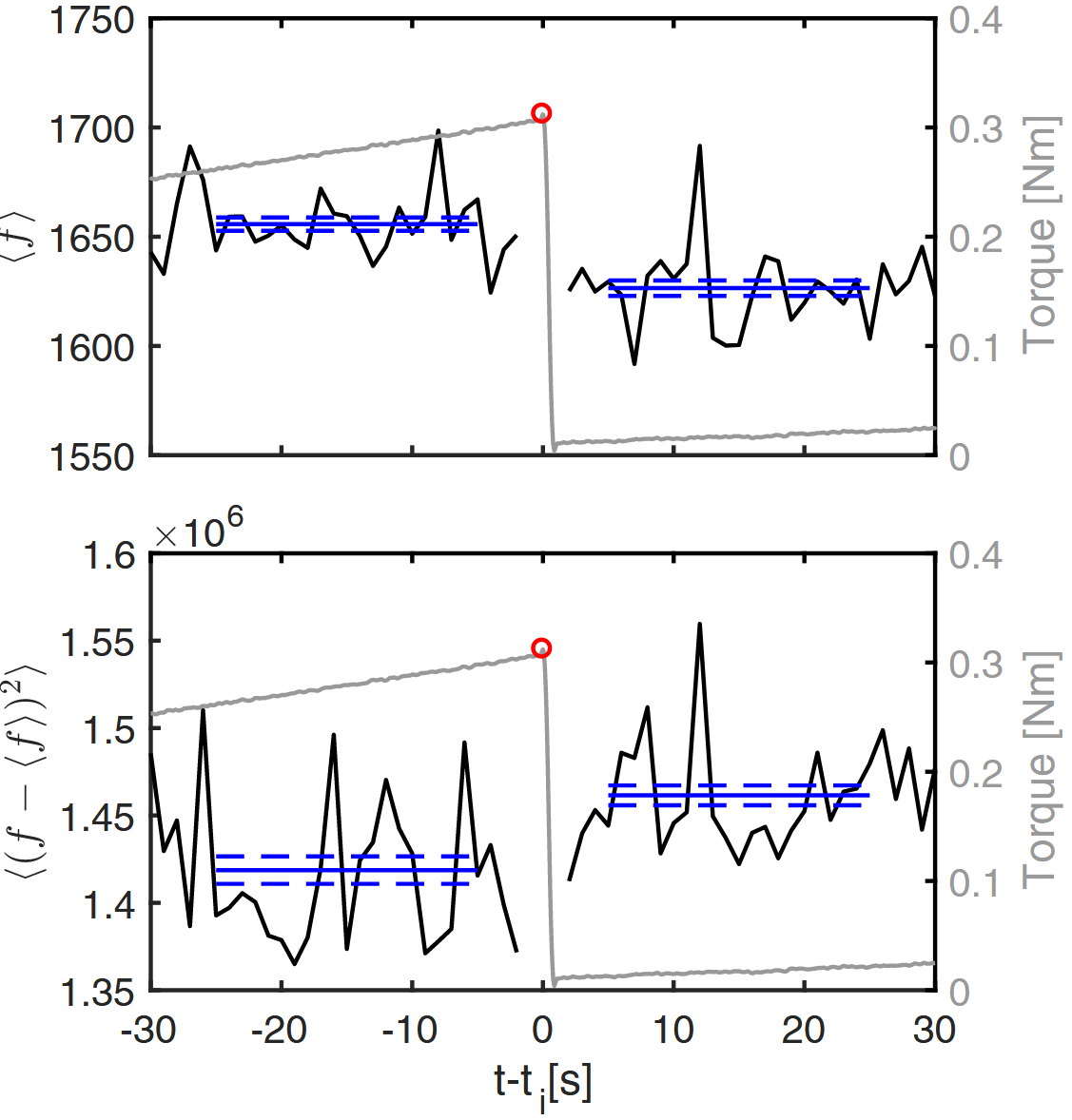
(top) $\langle f\rangle$ and (middle) $\langle(f-\langle f\rangle)^{2}\rangle$ for $D_{\text{ex}}(f;t-t_{i})$ for a single slip, measured by a single sensor. The solid blue lines show the mean values for the first and last $28$ seconds, respectively, and dashed lines show the $95\%$ confidence in these means. In both plots, the torque is plotted on the right axis in light grey, with the slip indicated by a red circle. (bottom) The success rates for which we observed statistically significant discontinuities in the mean, variance, and kurtosis in $f$ for $D_{\text{ex}}$ as measured by a single sensor and at a time coincident with a slip. Boldface values are those that match the sign of the average changes.
(上) $\langle f\rangle$ 和 (中) $\langle(f-\langle f\rangle)^{2}\rangle$ 的 $D_{\text{ex}}(f;t-t_{i})$,由单个传感器测量的单次滑移。蓝色实线分别表示前 $28$ 秒和后 $28$ 秒的平均值,虚线表示这些平均值的置信度为 $95\%$。在这两幅图中,扭矩都以浅灰色绘制在右轴上,滑移用红圈表示。 (下图) 我们观察到 $D_{\text{ex}}$f$ 的均值、方差和峰度在统计意义上存在显著不连续性的成功率,这些均值、方差和峰度由单个传感器测量,时间与滑移时间重合。粗体字数值与平均变化的符号一致。
The analysis we present here represents an important step in connecting passive acoustic measurements directly to the state of the material. While acoustic emissions have previously been known to coincide with the failure of granular media, our method provides a new capability: assessment of the progress of a system en route to failure. The shift observed in moments of the occupancy of vibrational modes is consistent with observations that granular systems under less stress exhibit an excess of floppy, low-frequency modes, and can be connected more broadly to similar observations in jammed solids as the volume fraction is reduced and as shear progresses.
我们在此提出的分析方法是将被动声学测量与材料状态直接联系起来的重要一步。以前人们知道声发射与颗粒介质的失效相吻合,而我们的方法提供了一种新的能力:评估系统在失效过程中的进展。观察到的振动模式占据时刻的变化与观察到的应力较小的颗粒系统表现出过多的软质、低频模式相一致,并且随着体积分数的降低和剪切力的增加,可以更广泛地与堵塞固体中的类似观察结果联系起来。
Our results indicate promise for predictive forecasting of failure in slowly sheared, disordered systems. However, any approach to forecasting of this sort is most likely to be probabilistic rather than deterministic: $\tilde{D}_{\text{ex}}$ may signal an increased likelihood for an event, particularly with better sensor coverage where passive measurements may more completely reveal the features of the density of vibrational modes. These techniques also provide a route for improved characterization of the vibrational properties of disordered materials.
我们的研究结果表明,在缓慢剪切的无序系统中,预测失效是有希望的。然而,任何此类预测方法都很可能是概率性的,而非确定性的:$\tilde{D}_{\text{ex}}$ 可能预示着事件发生的可能性增加,尤其是在传感器覆盖范围更广的情况下,被动测量可能会更全面地揭示振动模式密度的特征。这些技术还为改进无序材料振动特性的表征提供了一条途径。
Assessing the internal stress state of a granular system is notoriously difficult: photoelastic, optical, and tomographic techniques require specialized materials or slow scanning times to make quantitative measurements of internal stresses. We have found that the density of excited vibrational modes $D_{\text{ex}}(f)$ appears to provide a new technique for reporting the internal stress in the system which does not require optical access, and can be applied to 3D systems with fast measurement times.
评估颗粒系统的内应力状态是众所周知的难题:光弹性、光学和断层扫描技术需要专门的材料或缓慢的扫描时间才能对内应力进行定量测量。我们发现,激发振动模式的密度 $D_{\text{ex}}(f)$ 似乎提供了一种报告系统内应力的新技术,它不需要光学接入,而且可以快速测量三维系统。
Importantly, this method does not require acoustic driving, which risks triggering a failure in materials near threshold, and should work on a variety of materials. Furthermore, this analysis is largely independent of the details of the sensor mechanism, so an obvious next step is to test the approach with seismic data.
重要的是,这种方法不需要声波驱动,因为声波驱动有可能在接近(屈服)阈值的材料中引发失效,而且应该适用于各种材料。此外,这种分析在很大程度上与传感器机制的细节无关,因此下一步显然是用地震数据测试这种方法。