DOI: 10.1029/93JB02974
Abstract
A theoretical study of the propagation of a plane wave in a material with nonlinear response is presented. We start with the wave equation for an isotropic, homogeneous, elastic solid with cubic anharmonicity in the moduli, accounting for attenuation by introducing complex linear and nonlinear moduli. A heirarchy of equations, ordered in powers of the displacement field, is developed. Using a Green function technique, we solve this set of equations systematically for the displacement field at distance $x$ from the source. We examine the influence of propagation distance, source frequency spectrum, source displacement amplitude, attenuation, and nonlinear coefficient on the spectrum of a propagating wave. The displacement field for various source functions is calculated using parameters typical of rocks.
本文介绍了平面波在非线性响应材料中传播的理论研究。我们从模量为立方非谐波的各向同性均质弹性固体的波方程入手,通过引入复杂的线性和非线性模量来考虑衰减。我们建立了一个以位移场的幂次排列的方程体系。利用 Green 函数方法,我们系统地求解了与声源距离 $x$ 处的位移场方程组。我们研究了传播距离、源频谱、源位移振幅、衰减和非线性系数对传播波频谱的影响。我们使用岩石的典型参数计算了各种源函数的位移场。
Introduction
In this paper we consider the nonlinear interaction of frequency components in large-amplitude elastic waves in rocks. Compared to other, more ordered solids, rocks are highly elastically nonlinear. Because of the presence of structural defects such as microcracks and grain boundaries, the effective moduli in rocks change dramatically as a function of stress. The ratio of third-order elastic constants to second-order elastic constants in sandstone is typically orders of magnitude greater than in solids such as iron [Nazarov et al., 1988]. This high degree of nonlinearity means that frequency components mix and energy is transferred from the fundamental frequencies to sum and difference frequencies. We are currently interested in three potential applications of nonlinear effects in rocks.
(1) We are interested in modeling of explosion and earthquake sources, where we assume large amounts of energy are transferred from the source frequency spectrum to higher and lower frequencies. The received seismic frequency spectrum may be only distantly related to the original-source frequency spectrum.
(2) We are interested in creating a low-frequency seismic source by mixing two high-frequency sources. In general, the lower the frequency desired for a seismic survey, the larger the source must be.
(3) We are interested in measuring nonlinear coefficients of highly disordered solids like rocks. Consolidation and saturation conditions cause large deviations in the measured nonlinear coefficients of similar rocks. Therefore accurate measurement of nonlinear terms can be a sensitive measure of consolidation and saturation.
在本文中,我们考虑了岩石中大振幅弹性波频率成分的非线性相互作用。与其他更有序的固体相比,岩石具有高度的弹性非线性。由于微裂缝和晶界等结构缺陷的存在,岩石中的有效模量随应力的变化而急剧变化。砂岩中的三阶弹性常数与二阶弹性常数之比通常要比铁等固体大几个数量级[Nazarov 等人,1988 年]。这种高度非线性意味着频率成分混合,能量从基频转移到和频和差频。我们目前对岩石中非线性效应的三个潜在应用感兴趣。
(1) 我们对爆炸和地震源建模感兴趣,假设大量能量从震源频谱转移到较高和较低频率。接收到的地震频谱可能与原始震源频谱仅有很小的关系。
(2) 我们希望通过混合两个高频震源来产生低频震源。一般来说,地震勘测所需的频率越低,震源就必须越大。
(3) 我们对测量岩石等高度无序固体的非线性系数很感兴趣。固结和饱和条件会导致类似岩石的非线性系数测量值出现较大偏差。因此,精确测量非线性系数可以灵敏地测量固结和饱和度。
The purpose of this paper is to develop and illustrate a theoretical framework for investigating these problems that has conceptual clarity and is easy to implement numerically. In the next section we derive the equation of motion for the displacement field from an energy functional that is correct to third order in the strain. We introduce attenuation into the description of the displacemenftield through a model in which the displacement derivative has instantaneous and retarded (in time) components. This model is discussed in the appendix. The resulting equation of motion for the displacement field lets us classify the forces that drive the displacement field as linear elastic, linear attenuative, nonlinear elastic, or nonlinear attenuative.
本文的目的是开发和说明研究这些问题的理论框架,该框架概念清晰,易于数值计算。在下一节中,我们将从能量函数推导出位移场的运动方程,该能量函数在应变方面的正确性达到了三阶。我们通过一个位移导数具有瞬时和延迟(时间)分量的模型,将衰减引入位移场的描述中。该模型将在附录中讨论。根据位移场的运动方程,我们可以将驱动位移场的力分为线性弹性力、线性衰减力、非线性弹性力或非线性衰减力。
We solve the equation of motion for the displacement field by developing the solution in terms of the exact solution of the linear problem. Thus we employ a Green function technique. We illustrate use of this technique in the general solution section, where we work through the case of plane waves propagating with linear elasticity, linear attenuation, nonlinear elasticity(cubic anharmonicity), and nonlinear attenuation. The analytic structure of the equation suggests the following physical description of the phenomena.
(1) The system is initially disturbed by an external source, e.g., a transducer at the origin. (2) The Green function describes propagation of the displacement field resulting from this disturbance into the interior of the system. (3) In the interior of the system, the nonlinearity acts on the displacement field to produce an internal source. (4) The Green function works again to carry the displacement consequences of this internal source to the detector.
我们根据线性问题的精确解来求解位移场的运动方程。因此,我们采用了 Green 函数方法。在一般求解部分,我们将通过线性弹性、线性衰减、非线性弹性(三次方非谐波)和非线性衰减的平面波传播情况来说明这一方法的使用。方程的解析结构表明对这些现象的物理描述如下:
(1) 系统最初受到外部干扰源的干扰,例如原点处的传感器。(2) Green 函数描述了干扰产生的位移场向系统内部的传播。(3) 在系统内部,非线性作用于位移场,产生内源。(4) Green 函数再次起作用,将这一内部源的位移后果传递给探测器。
This physical picture lends itself to generalization. For example, the retarded component of the stress field is quite possibly characterized by a spectrum of relaxation rates[Day and Minster, 1984]. The Green function for the corresponding linear problem is relatively complicated.However, there are well-known procedures for constructing an average Green function that faithfully describes such a circumstance. This Green function can be inserted into the relevant equations in place of the exact Green function with no other changes in the structure of the solution.
这种物理现象本身就具有概括性。例如,应力场的延迟分量很可能以弛豫率谱为特征[Day 和 Minster, 1984]。相应线性问题的 Green 函数相对复杂。不过,有一些众所周知的手法可以构建一个平均 Green 函数,忠实地描述这种情况。这个 Green 函数可以插入到相关方程中,代替精确的 Green 函数,并且不会改变解的结构。
The section on specific solution contains a description of a specific Green function for an infinite medium and the resulting displacement components to first order in the nonlinearity. In the section of examples we describe analytical and numerical results for nonlinear wave propagation in two realistic physical situations. In the first example we use a continuous sine wave source to derive an analytic displacementto first order in the nonlinearity. In the limit of low attenuation, these results agree with those of Polyakova[1964] and others. In the second example we use a broadband source to study the effect of nonlinear responseon seismic propagation. A summary of our conclusions is given in the final section.
具体解法部分描述了无限介质的具体 Green 函数以及由此产生的一阶非线性位移分量。在示例部分,我们描述了两种实际物理情况下非线性波传播的分析和数值结果。在第一个例子中,我们使用一个连续的正弦波源,得出非线性一阶位移的分析结果。在低衰减极限下,这些结果与 Polyakova[1964] 等人的研究结果一致。在第二个例子中,我们使用宽带震源来研究非线性响应对地震传播的影响。最后一节对我们的结论进行了总结。
Formulation of Problem
The derivation of the equations of motion for a homogeneous solid, including first-order nonlinear elastic terms and linear attenuation,has been described many times. In order to be complete and to fix notation, we sketch a synthesis of the derivations presented by Landau and Lifshitz[1959], Murnaghan[1951], Polyakova [1964], and Green[1973].
均质固体运动方程的推导,包括一阶非线性弹性项和线性衰减,已被多次描述。为了完整和固定符号,我们对 Landau 和 Lifshitz[1959]、Murnaghan[1951]、Polyakova[1964]以及 Green[1973]的推导进行了综合。
The equation of motion for elastic wave propagation is
$$ \begin{equation} \rho \ddot{u}_{i} = \partial \sigma_{ij} / \partial x_{j},\tag{1}\label{eq:1} \end{equation} $$
where $\rho$ is the density of the undeformed solid, $u_{i}$ is the particle displacemen at long coordinate $i$, $\sigma_{ij}$ is the $i$ $j$ component of the stress tensor, and $x_{j}$ is the $j$th coordinate. Conventional summation notation is used. The stress tensor is given by
$$ \begin{equation} \sigma_{ij} = \frac{\partial \varepsilon}{\partial(\partial u_{i}/\partial x_{j})}, \tag{2}\label{eq:2} \end{equation} $$
where $\varepsilon$ is the internal energy density of a homogeneous, elastic solid. Including third-order terms in the strain, the internal energy density may be written
$$ \begin{equation} \varepsilon = \frac{\lambda+2\mu}{2}I_{1}^{2} - 2\mu I_{2} + \frac{l+2m}{3}I_{1}^{3} - 2mI_{1}I_{2} + nI_{3}, \tag{3}\label{eq:3} \end{equation} $$
where $\lambda$ and $\mu$ are second-order elastic constants(Lame coefficients); $l$, $m$, and $n$ are third-order elastic constants(Murnaghan coefficients); and $I_{1}$, $I_{2}$, $I_{3}$ are the three invariants of the strain tensor:
$$ \begin{equation} \begin{aligned} I_{1} &= \varepsilon_{ii},\\ I_{2} &= \left|\begin{matrix} \varepsilon_{22} & \varepsilon_{23}\\ \varepsilon_{32} & \varepsilon_{33}\end{matrix}\right| + \left|\begin{matrix} \varepsilon_{33} & \varepsilon_{31}\\ \varepsilon_{13} & \varepsilon_{11}\end{matrix}\right| + \left|\begin{matrix} \varepsilon_{11} & \varepsilon_{12}\\ \varepsilon_{21} & \varepsilon_{22}\end{matrix}\right|,\\ I_{3} &= \text{det}\varepsilon_{ij}, \end{aligned} \tag{4}\label{eq:4} \end{equation} $$
where the components of the strain tensor are given by
$$ \begin{equation} \varepsilon_{ij} = \frac{1}{2}\left(\frac{\partial u_{i}}{\partial x_{j}} + \frac{\partial u_{j}}{\partial x_{i}} + \frac{\partial u_{k}}{\partial x_{i}}\frac{\partial u_{k}}{\partial u_{j}}\right). \tag{5}\label{eq:5} \end{equation} $$
弹性波传播的运动方程为
$$ \begin{equation} \rho \ddot{u}_{i} = \partial \sigma_{ij} / \partial x_{j},\tag{1} \end{equation} $$
其中 $\rho$ 为未形变固体的密度,$u_{i}$ 为粒子在长坐标 $i$ 处的位移,$\sigma_{ij}$ 为应力张量的 $i$ $j$ 分量,$x_{j}$ 为第 $j$ 个坐标。这里使用的是传统的求和符号。应力张量的计算公式为
$$ \begin{equation} \sigma_{ij} = \frac{\partial \varepsilon}{\partial(\partial u_{i}/\partial x_{j})}, \tag{2} \end{equation} $$
其中 $\varepsilon$ 是均质弹性固体的内能密度。若包括应变的三阶项,内能密度可写成
$$ \begin{equation} \varepsilon = \frac{\lambda+2\mu}{2}I_{1}^{2} - 2\mu I_{2} + \frac{l+2m}{3}I_{1}^{3} - 2mI_{1}I_{2} + nI_{3}, \tag{3} \end{equation} $$
其中,$\lambda$ 和 $\mu$ 是二阶弹性常数(Lame 系数);$l$、$m$ 和 $n$ 是三阶弹性常数(Murnaghan 系数);$I_{1}$、$I_{2}$ 和 $I_{3}$ 是应变张量的三个不变量:
$$ \begin{equation} \begin{aligned} I_{1} &= \varepsilon_{ii},\\ I_{2} &= \left|\begin{matrix} \varepsilon_{22} & \varepsilon_{23}\\ \varepsilon_{32} & \varepsilon_{33}\end{matrix}\right| + \left|\begin{matrix} \varepsilon_{33} & \varepsilon_{31}\\ \varepsilon_{13} & \varepsilon_{11}\end{matrix}\right| + \left|\begin{matrix} \varepsilon_{11} & \varepsilon_{12}\\ \varepsilon_{21} & \varepsilon_{22}\end{matrix}\right|,\\ I_{3} &= \text{det}\varepsilon_{ij}, \end{aligned} \tag{4} \end{equation} $$
其中应变张量的分量为
$$ \begin{equation} \varepsilon_{ij} = \frac{1}{2}\left(\frac{\partial u_{i}}{\partial x_{j}} + \frac{\partial u_{j}}{\partial x_{i}} + \frac{\partial u_{k}}{\partial x_{i}}\frac{\partial u_{k}}{\partial u_{j}}\right). \tag{5} \end{equation} $$
For simplicity, we restrict ourselves to the problem of wave propagation in a single direction, the $x$ direction. Combining $\eqref{eq:1}$-$\eqref{eq:5}$ and keeping terms to second order in the displacement field, the equations of motion for the displacemen fiteld are [Gol’dberg, 1960]:
$$ \begin{equation} \begin{aligned} \rho\ddot{u}_{x} &= (\lambda+2\mu)\frac{\partial^{2}u_{x}}{\partial x^{2}} + S_{x}^{\prime}\\ & + \frac{1}{2}[3(\lambda+2\mu) + 2(l + 2m)]\frac{\partial}{\partial x}\left(\frac{\partial u_{x}}{\partial x}\right)^{2}\\ & + \frac{1}{2}(\lambda + 2\mu + m)\frac{\partial}{\partial x}\left[\left(\frac{\partial u_{y}}{\partial x}\right)^{2} + \left(\frac{\partial u_{z}}{\partial x}\right)^{2}\right], \end{aligned}\tag{6a}\label{eq:6a}\\ \end{equation} $$ $$ \begin{equation} \begin{aligned} \rho\ddot{u}_{y} = \mu\frac{\partial^{2} u_{y}}{\partial x^{2}} + S_{y}^{\prime} + (\lambda + 2\mu + m)\frac{\partial}{\partial x}\left(\frac{\partial u_{x}}{\partial x}\frac{\partial u_{y}}{\partial x}\right), \end{aligned}\tag{6b}\label{eq:6b}\\ \end{equation} $$ $$ \begin{equation} \begin{aligned} \rho\ddot{u}_{z} = \mu\frac{\partial^{2} u_{z}}{\partial x^{2}} + S_{z}^{\prime} + (\lambda + 2\mu + m)\frac{\partial}{\partial x}\left(\frac{\partial u_{x}}{\partial x}\frac{\partial u_{z}}{\partial x}\right), \end{aligned}\tag{6c}\label{eq:6c} \end{equation} $$
Here $S_{i}^{\prime}(x,t)$ is the external source that initiates the response of the system. These equations describe a system having linear and nonlinear elasticity(cubic anharmonicity).
为简单起见,我们只讨论波在单一方向(即 $x$ 方向)的传播问题。结合 $\eqref{eq:1}$-$\eqref{eq:5}$ 并在位移场中保持二阶项,位移场的运动方程为[Gol’dberg, 1960]:
$$ \begin{equation} \begin{aligned} \rho\ddot{u}_{x} &= (\lambda+2\mu)\frac{\partial^{2}u_{x}}{\partial x^{2}} + S_{x}^{\prime}\\ & + \frac{1}{2}[3(\lambda+2\mu) + 2(l + 2m)]\frac{\partial}{\partial x}\left(\frac{\partial u_{x}}{\partial x}\right)^{2}\\ & + \frac{1}{2}(\lambda + 2\mu + m)\frac{\partial}{\partial x}\left[\left(\frac{\partial u_{y}}{\partial x}\right)^{2} + \left(\frac{\partial u_{z}}{\partial x}\right)^{2}\right], \end{aligned}\tag{6a}\\ \end{equation} $$ $$ \begin{equation} \begin{aligned} \rho\ddot{u}_{y} = \mu\frac{\partial^{2} u_{y}}{\partial x^{2}} + S_{y}^{\prime} + (\lambda + 2\mu + m)\frac{\partial}{\partial x}\left(\frac{\partial u_{x}}{\partial x}\frac{\partial u_{y}}{\partial x}\right), \end{aligned}\tag{6b}\\ \end{equation} $$ $$ \begin{equation} \begin{aligned} \rho\ddot{u}_{z} = \mu\frac{\partial^{2} u_{z}}{\partial x^{2}} + S_{z}^{\prime} + (\lambda + 2\mu + m)\frac{\partial}{\partial x}\left(\frac{\partial u_{x}}{\partial x}\frac{\partial u_{z}}{\partial x}\right), \end{aligned}\tag{6c} \end{equation} $$
这里,$S_{i}^{\prime}(x,t)$ 是引发系统响应的外部源。这些方程描述了一个具有线性和非线性弹性(三次谐波)的系统。
In the frequency domain an explicit Green function can be found for the problem involving linear elasticity and linear attenuation. Therefore define $u_{i}(x,\omega)$ and $S_{i}^{\prime}(x,\omega)$ such that
$$ \begin{align} u_{i}(x,t) &= \int_{-\infty}^{+\infty}\frac{\mathrm{d}\omega}{2\pi}u_{i}(x,\omega)e^{-i\omega t},\tag{7a}\label{eq:7a}\\ S_{i}^{\prime}(x,t) &= \int_{-\infty}^{+\infty}\frac{\mathrm{d}\omega}{2\pi}S_{i}^{\prime}(x,\omega)e^{-i\omega t}.\tag{7b}\label{eq:7b} \end{align} $$
We introduce attenuation by allowing the spatial derivative of the displacement to have a component that is retarded in time (see the appendix). We let
$$ \begin{equation} \frac{\partial u_{i}(x,\omega)}{\partial x}\rightarrow \chi(\omega)\frac{\partial u_{i}(x,\omega)}{\partial x},\tag{8}\label{eq:8} \end{equation} $$
where
$$ \begin{equation} \chi(\omega) = 1 - \frac{\Delta}{1 - \text{sgn}(\omega)i|\omega\tau|^{\nu}},\tag{9}\label{eq:9} \end{equation} $$
$\Delta$ can be thought of as the fractional amount of the displacement derivative that is retarded in time ($0\leq \Delta \leq 1$), and $\tau$ is the characteristic damping time. In the linear case the factor $\chi(\omega)$ is equivalent to the complex factor multiplying real moduli in the standard solid model of a series Voigt unit and spring[Nowick and Berry, 1972], that is, $M\rightarrow \chi(\omega)M$, where $M$ is a modulus. We have made a generalization of the standard form by adding the power $\nu$.
在频域中,可以为涉及线性弹性和线性衰减的问题找到显式 Green 函数。因此,定义 $u_{i}(x,\omega)$ 和 $S_{i}^{\prime}(x,\omega)$ ,使得
$$ \begin{align} u_{i}(x,t) &= \int_{-\infty}^{+\infty}\frac{\mathrm{d}\omega}{2\pi}u_{i}(x,\omega)e^{-i\omega t},\tag{7a}\\ S_{i}^{\prime}(x,t) &= \int_{-\infty}^{+\infty}\frac{\mathrm{d}\omega}{2\pi}S_{i}^{\prime}(x,\omega)e^{-i\omega t}.\tag{7b} \end{align} $$
我们通过允许位移的空间导数在时间上具有滞后分量来引入衰减(见 Appendix )。我们让
$$ \begin{equation} \frac{\partial u_{i}(x,\omega)}{\partial x}\rightarrow \chi(\omega)\frac{\partial u_{i}(x,\omega)}{\partial x},\tag{8} \end{equation} $$
其中
$$ \begin{equation} \chi(\omega) = 1 - \frac{\Delta}{1 - \text{sgn}(\omega)i|\omega\tau|^{\nu}},\tag{9} \end{equation} $$
$$ \begin{equation*} \text{sgn}(\omega) = \begin{cases} 1, & \omega > 0,\\ 0, & \omega = 0,\\ -1, & \omega < 0\end{cases} \end{equation*} $$
$\Delta$ 可以看作是位移导数在时间上延迟的分数($0\leq \Delta \leq 1$),$\tau$ 是特征阻尼时间。在线性情况下,系数 $\chi(\omega)$ 等同于串联 Voigt 单元或弹簧的标准实体模型中的复系数乘以实模量[Nowick and Berry, 1972],即 $M\rightarrow \chi(\omega)M$, 其中 $M$ 为模量。我们通过添加幂 $\nu$ 对标准形式进行了概括。
To be more general, we could allow the complex part of $\chi$ to depend on the displacement component. By making the assumption that $\tau$, $\nu$, and $\Delta$ are the same for all displacement components,we are making the assumptions that the dimensionless measure of anelasticity $Q$ of the system is the same for both compressional and shear waves and that both types of waves experience the same velocity shift from low to high frequency. Defining $Q^{-1} = -\text{Im}(\chi)/\text{Re}(\chi)$ [O’Connell and Budiansky, 1978], we find
$$ Q^{-1} = \frac{\text{sgn}(\omega)\Delta|\omega\tau|^{\nu}}{1 - \Delta + |\omega\tau|^{2\nu}}.\tag{10}\label{eq:10} $$
For $\nu = 0$, we find a constant $Q$ result. For $\nu\neq 0$, the linear moduli and $Q$ have low- and high-frequency limits. For lowfrequencies, $|\omega\tau|\ll 1$,
$$ \begin{equation} \chi(\omega) \rightarrow (1 - \Delta) - \text{sgn}(\omega)i|\omega\tau|^{\nu}\Delta, \tag{11a}\label{eq:11a} \end{equation} $$
and $Q^{-1}\rightarrow \text{sgn}(\omega)|\omega\tau|^{\nu}\Delta/(1-\Delta)$. For high frequencies, $|\omega\tau|\gg 1$,
$$ \begin{equation} \chi(\omega)\rightarrow 1 - \text{sgn}(\omega)i|\omega\tau|^{-\nu}\Delta \tag{11b}\label{eq:11b} \end{equation} $$
and $Q^{-1}\rightarrow \text{sgn}(\omega)|\omega\tau|^{-\nu}\Delta$. In both limits the linear moduli have a small residual complex component. At low frequency the real linear moduli are a factor of $1-\Delta$ smaller than at high frequency. The parameters $\Delta$, $\tau$, and $\nu$ maybe derived from measurements of $Q^{-1}$ as a function of frequency.
为了更普遍,我们可以允许 $\chi$ 的复数部分取决于位移分量。通过假设所有位移分量的 $\tau$、$\nu$ 和 $\Delta$ 都是相同的,我们可以假设系统的无量纲弹性度量 $Q$ 对于压缩波和剪切波都是相同的,并且两种波从低频到高频都经历了相同的速度偏移。定义 $Q^{-1} = -\text{Im}(\chi)/\text{Re}(\chi)$ [O’Connell 和 Budiansky, 1978], 我们发现
$$ Q^{-1} = \frac{\text{sgn}(\omega)\Delta|\omega\tau|^{\nu}}{1 - \Delta + |\omega\tau|^{2\nu}}.\tag{10} $$
对于 $\nu = 0$,我们发现 $Q$ 为定值。对于 $\nu\neq 0$,线性模量和 $Q$ 有低频和高频极限。对于低频,$|\omega\tau|\ll 1$,
$$ \begin{equation} \chi(\omega) \rightarrow (1 - \Delta) - \text{sgn}(\omega)i|\omega\tau|^{\nu}\Delta, \tag{11a} \end{equation} $$
并且 $Q^{-1}\rightarrow \text{sgn}(\omega)|\omega\tau|^{\nu}\Delta/(1-\Delta)$. 对于高频率,$|\omega\tau|\gg 1$,
$$ \begin{equation} \chi(\omega)\rightarrow 1 - \text{sgn}(\omega)i|\omega\tau|^{-\nu}\Delta \tag{11b} \end{equation} $$
和 $Q^{-1}\rightarrow \text{sgn}(\omega)|\omega\tau|^{-\nu}\Delta$. 在这两个极限中,线性模量都有一个很小的残余复数分量。在低频下,实线性模量比高频下小 $1-\Delta$ 倍。参数 $\Delta$、$\tau$ 和 $\nu$ 可能是通过测量 $Q^{-1}$ 与频率的函数关系得出的。
General Solution Using Green Function
We write the equations of longitudinal(L) and transverse(T) motion, $\eqref{eq:6a}$-$\eqref{eq:6c}$, in the frequency domain by using the relation for attenuation in $\eqref{eq:8}$, the Fourier transforms of $\eqref{eq:7a}$ and $\eqref{eq:7b}$, and the convolution theorem for Fourier transforms. The equations of motion are
$$ \begin{align} &g_{L}^{-1}(x,\omega)u_{x}(x,\omega) = -S_{x}(x,\omega) - \beta\frac{\partial}{\partial x}\int\frac{\mathrm{d}\omega^{\prime}}{2\pi}\chi(\omega^{\prime})\chi(\phi)\frac{\partial u_{x}(x,\omega^{\prime})}{\partial x}\frac{\partial u_{x}(x,\phi)}{\partial x} \\ &-\gamma\frac{\partial}{\partial x}\int\frac{\mathrm{d}\omega^{\prime}}{2\pi}\chi(\omega^{\prime})\chi(\phi)\left[\frac{\partial u_{y}(x,\omega^{\prime})}{\partial x}\frac{\partial u_{y}(x,\phi)}{\partial x} + \frac{\partial u_{z}(x,\omega^{\prime})}{\partial x}\frac{\partial u_{z}(x,\phi)}{\partial x}\right],\tag{12a}\label{eq:12a}\\ &g_{T}^{-1}(x,\omega)u_{y}(x,\omega) = -S_{y}(x,\omega) - 2\gamma\frac{c_{L}^{2}}{c_{T}^{2}}\frac{\partial}{\partial x}\int\frac{\mathrm{d}\omega^{\prime}}{2\pi}\chi(\omega^{\prime})\chi(\phi)\frac{\partial u_{x}(x,\omega^{\prime})}{\partial x}\frac{\partial u_{y}(x,\phi)}{\partial x},\tag{12b}\label{eq:12b}\\ &g_{T}^{-1}(x,\omega)u_{z}(x,\omega) = -S_{z}(x,\omega)-2\gamma\frac{c_{L}^{2}}{c_{T}^{2}}\frac{\partial}{\partial x}\int\frac{\mathrm{d}\omega^{\prime}}{2\pi}\chi(\omega^{\prime})\chi(\phi)\frac{\partial u_{x}(x,\omega^{\prime})}{\partial x}\frac{\partial u_{z}(x,\phi)}{\partial x},\tag{12c}\label{eq:12c} \end{align} $$
where
$$ \begin{align} &g_{L}^{-1}(x,\omega) = \chi(\omega)\frac{\partial^{2}}{\partial x^{2}} + k_{L}^{2},\tag{13a}\label{eq:13a}\\ &g_{T}^{-1}(x,\omega) = \chi(\omega)\frac{\partial^{2}}{\partial x^{2}} + k_{T}^{2},\tag{13b}\label{eq:13b}\\ &\beta = \frac{3(\lambda + 2\mu) + 2(l + 2m)}{2(\lambda + 2\mu)},\tag{14a}\label{eq:14a}\\ &\gamma = \frac{\lambda + 2\mu + m}{2(\lambda + 2\mu)},\tag{14b}\label{eq:14b} \end{align} $$
$k_{L}^{2} = \omega^{2}/c_{L}^{2}$, $k_{T}^{2} = \omega^{2}/c_{T}^{2}$, $c_{L}^{2} = (\lambda + 2\mu)/\rho$, $c_{T}^{2} = \mu/\rho$, $S_{i} = S_{i}^{\prime}/(\lambda + 2\mu)$, and $\phi = \omega - \omega^{\prime}$. The linear terms in the equations of motion, $\eqref{eq:12a}$-$\eqref{eq:12c}$, are on the left-hand side in the operator $g_{L}^{-1}$ and $g_{T}^{-1}$. The right-hand sides of $\eqref{eq:12a}$-$\eqref{eq:12c}$ have two kinds of sources, the external sources $S_{i}(x,\omega)$ and the internal sources due to the nonlinearity.
我们利用 $\eqref{eq:8}$ 中的衰减关系、$\eqref{eq:7a}$ 和 $\eqref{eq:7b}$ 的傅里叶变换以及傅里叶变换的卷积定理,在频域中写出了纵向(L)和横向(T)运动方程 $\eqref{eq:6a}$-$\eqref{eq:6c}$ 。运动方程为
$$ \begin{align} &g_{L}^{-1}(x,\omega)u_{x}(x,\omega) = -S_{x}(x,\omega) - \beta\frac{\partial}{\partial x}\int\frac{\mathrm{d}\omega^{\prime}}{2\pi}\chi(\omega^{\prime})\chi(\phi)\frac{\partial u_{x}(x,\omega^{\prime})}{\partial x}\frac{\partial u_{x}(x,\phi)}{\partial x} \\ &-\gamma\frac{\partial}{\partial x}\int\frac{\mathrm{d}\omega^{\prime}}{2\pi}\chi(\omega^{\prime})\chi(\phi)\left[\frac{\partial u_{y}(x,\omega^{\prime})}{\partial x}\frac{\partial u_{y}(x,\phi)}{\partial x} + \frac{\partial u_{z}(x,\omega^{\prime})}{\partial x}\frac{\partial u_{z}(x,\phi)}{\partial x}\right],\tag{12a}\\ &g_{T}^{-1}(x,\omega)u_{y}(x,\omega) = -S_{y}(x,\omega) - 2\gamma\frac{c_{L}^{2}}{c_{T}^{2}}\frac{\partial}{\partial x}\int\frac{\mathrm{d}\omega^{\prime}}{2\pi}\chi(\omega^{\prime})\chi(\phi)\frac{\partial u_{x}(x,\omega^{\prime})}{\partial x}\frac{\partial u_{y}(x,\phi)}{\partial x},\tag{12b}\\ &g_{T}^{-1}(x,\omega)u_{z}(x,\omega) = -S_{z}(x,\omega)-2\gamma\frac{c_{L}^{2}}{c_{T}^{2}}\frac{\partial}{\partial x}\int\frac{\mathrm{d}\omega^{\prime}}{2\pi}\chi(\omega^{\prime})\chi(\phi)\frac{\partial u_{x}(x,\omega^{\prime})}{\partial x}\frac{\partial u_{z}(x,\phi)}{\partial x},\tag{12c} \end{align} $$
其中
$$ \begin{align} &g_{L}^{-1}(x,\omega) = \chi(\omega)\frac{\partial^{2}}{\partial x^{2}} + k_{L}^{2},\tag{13a}\\ &g_{T}^{-1}(x,\omega) = \chi(\omega)\frac{\partial^{2}}{\partial x^{2}} + k_{T}^{2},\tag{13b}\\ &\beta = \frac{3(\lambda + 2\mu) + 2(l + 2m)}{2(\lambda + 2\mu)},\tag{14a}\\ &\gamma = \frac{\lambda + 2\mu + m}{2(\lambda + 2\mu)},\tag{14b} \end{align} $$
$k_{L}^{2} = \omega^{2}/c_{L}^{2}$, $k_{T}^{2} = \omega^{2}/c_{T}^{2}$, $c_{L}^{2} = (\lambda + 2\mu)/\rho$、$c_{T}^{2} = \mu/\rho$, $S_{i} = S_{i}^{\prime}/(\lambda + 2\mu)$, $\phi = \omega - \omega^{\prime}$.运动方程中的线性项 $\eqref{eq:12a}$-$\eqref{eq:12c}$ 位于算子 $g_{L}^{-1}$ 和 $g_{T}^{-1}$ 的左侧。$\eqref{eq:12a}$-$\eqref{eq:12c}$ 的右边有两种来源,一种是外部来源 $S_{i}(x,\omega)$,另一种是非线性导致的内部来源。
To obtain a systematic Green function solution to $\eqref{eq:12a}$-$\eqref{eq:12c}$, we use a parameter $\eta(0<\eta\leq 1)$ to keep track of powers of the internal source. We expand the displacement and source functions in powers of $\eta$;
$$ \begin{align} u_{i}(x,\omega) = u_{i}^{(0)}(x,\omega) + \eta u_{i}^{(1)}(x,\omega) + \eta^{2}u_{i}^{(2)}(x,\omega) + \cdots, \tag{15a}\label{eq:15a}\\ f_{i}(x,\omega) = f_{i}^{(0)}(x,\omega) + \eta f_{i}^{(1)}(x,\omega) + \eta^{2}f_{i}^{(2)}(x,\omega) + \cdots, \tag{15b}\label{eq:15b} \end{align} $$
where $f_{i}^{(0)}(x,\omega)$ is the external source function $S_{i}(x,\omega)$. In the examples we set $\eta\equiv 1$ and consider only cases where $|u_{i}^{(n+1)}|/|u_{i}^{(n)}| < 1$ and the expansion for $u_{i}$ is convergent. The first few terms in the expansion of the source function are given by
$$ \begin{align} f_{x}^{(0)}(x,\omega) &= S_{x}(x,\omega),\tag{16a}\label{eq:16a}\\ f_{x}^{(0)}(x,\omega) &= \frac{\partial}{\partial x}\int\frac{\mathrm{d}\omega^{\prime}}{2\pi}\chi(\omega^{\prime})\chi(\phi)\left\{\gamma\left[\frac{\partial u_{y}^{(0)}(x,\omega^{\prime})}{\partial x}\frac{\partial u_{y}^{(0)}(x,\phi)}{\partial x} + \frac{\partial u_{z}^{(0)}(x,\omega^{\prime})}{\partial x}\frac{\partial u_{z}^{(0)}(x,\phi)}{\partial x}\right] + \beta\frac{\partial u_{x}^{(0)}(x,\omega^{\prime})}{\partial x}\frac{\partial u_{x}^{(0)}(x,\phi)}{\partial x}\right\},\tag{16b}\label{eq:16b}\\ f_{x}^{(2)}(x,\omega) &= \frac{\partial}{\partial x}\int\frac{\mathrm{d}\omega^{\prime}}{2\pi}\chi(\omega^{\prime})\chi(\phi)\left\{2\gamma\left[\frac{\partial u_{y}^{(0)}(x,\omega^{\prime})}{\partial x}\frac{\partial u_{y}^{(1)}(x,\phi)}{\partial x} + \frac{\partial u_{z}^{(0)}(x,\omega^{\prime})}{\partial x}\frac{\partial u_{z}^{(1)}(x,\phi)}{\partial x}\right] + 2\beta\frac{\partial u_{x}^{(0)}(x,\omega^{\prime})}{\partial x}\frac{\partial u_{x}^{(1)}(x,\phi)}{\partial x}\right\},\tag{16c}\label{eq:16c}\\ f_{y}^{(0)}(x,\omega) &= S_{y}(x,\omega),\tag{16d}\label{eq:16d}\\ f_{y}^{(1)}(x,\omega) &= \frac{\partial }{\partial x}\int\frac{\mathrm{d}\omega^{\prime}}{2\pi}\chi(\omega^{\prime})\chi(\phi)\cdot 2\gamma\frac{c_{L}^{2}}{c_{T}^{2}}\frac{\partial u_{x}^{(0)}(x,\omega^{\prime})}{\partial x}\frac{\partial u_{y}^{(0)}(x,\phi)}{\partial x},\tag{16e}\label{eq:16e}\\ f_{y}^{(2)}(x,\omega) &= \frac{\partial}{\partial x}\int\frac{\mathrm{d}\omega^{\prime}}{2\pi}\chi(\omega^{\prime})\chi(\phi)\cdot 2\gamma\frac{c_{L}^{2}}{c_{T}^{2}}\left[\frac{\partial u_{x}^{(0)}(x,\omega^{\prime})}{\partial x}\frac{\partial u_{y}^{(1)}(x,\omega^{\prime})}{\partial x} + \frac{\partial u_{x}^{(1)}(x,\omega^{\prime})}{\partial x}\frac{\partial u_{y}^{(0)}(x,\phi)}{\partial x}\right],\tag{16f}\label{eq:16f} \end{align} $$
etc. Equating like powers of $\eta$, we obtain a hierarchy of equations that allows us to solve for the displacement field to any desired order:
$$ \begin{align} g_{L}^{-1}u_{x}^{(n)}(x,\omega) &= -f_{x}^{(n)}(x,\omega),\tag{17a}\label{eq:17a}\\ g_{T}^{-1}u_{j}^{(n)}(x,\omega) &= -f_{j}^{(n)}(x,\omega),\quad j=y,z. \tag{17b}\label{eq:17b} \end{align} $$
为了得到 $\eqref{eq:12a}$-$\eqref{eq:12c}$ 的 系统 Green 函数解,我们使用参数 $\eta$ $(0<\eta\leq 1)$ 来跟踪内部源的幂。我们用 $\eta$ 的幂来展开位移和源函数;
$$ \begin{align} u_{i}(x,\omega) = u_{i}^{(0)}(x,\omega) + \eta u_{i}^{(1)}(x,\omega) + \eta^{2}u_{i}^{(2)}(x,\omega) + \cdots, \tag{15a}\\ f_{i}(x,\omega) = f_{i}^{(0)}(x,\omega) + \eta f_{i}^{(1)}(x,\omega) + \eta^{2}f_{i}^{(2)}(x,\omega) + \cdots, \tag{15b} \end{align} $$
其中 $f_{i}^{(0)}(x,\omega)$ 是外部源函数 $S_{i}(x,\omega)$。在示例中,我们设置 $\eta\equiv 1$,并且只考虑 $|u_{i}^{(n+1)}|/|u_{i}^{(n)}| < 1$且 $u_{i}$ 的级数展开是收敛的情况。源函数展开的前几项由以下公式给出:
$$ \begin{align} f_{x}^{(0)}(x,\omega) &= S_{x}(x,\omega),\tag{16a}\\ f_{x}^{(0)}(x,\omega) &= \frac{\partial}{\partial x}\int\frac{\mathrm{d}\omega^{\prime}}{2\pi}\chi(\omega^{\prime})\chi(\phi)\left\{\gamma\left[\frac{\partial u_{y}^{(0)}(x,\omega^{\prime})}{\partial x}\frac{\partial u_{y}^{(0)}(x,\phi)}{\partial x} + \frac{\partial u_{z}^{(0)}(x,\omega^{\prime})}{\partial x}\frac{\partial u_{z}^{(0)}(x,\phi)}{\partial x}\right] + \beta\frac{\partial u_{x}^{(0)}(x,\omega^{\prime})}{\partial x}\frac{\partial u_{x}^{(0)}(x,\phi)}{\partial x}\right\},\tag{16b}\\ f_{x}^{(2)}(x,\omega) &= \frac{\partial}{\partial x}\int\frac{\mathrm{d}\omega^{\prime}}{2\pi}\chi(\omega^{\prime})\chi(\phi)\left\{2\gamma\left[\frac{\partial u_{y}^{(0)}(x,\omega^{\prime})}{\partial x}\frac{\partial u_{y}^{(1)}(x,\phi)}{\partial x} + \frac{\partial u_{z}^{(0)}(x,\omega^{\prime})}{\partial x}\frac{\partial u_{z}^{(1)}(x,\phi)}{\partial x}\right] + 2\beta\frac{\partial u_{x}^{(0)}(x,\omega^{\prime})}{\partial x}\frac{\partial u_{x}^{(1)}(x,\phi)}{\partial x}\right\},\tag{16c}\\ f_{y}^{(0)}(x,\omega) &= S_{y}(x,\omega),\tag{16d}\\ f_{y}^{(1)}(x,\omega) &= \frac{\partial }{\partial x}\int\frac{\mathrm{d}\omega^{\prime}}{2\pi}\chi(\omega^{\prime})\chi(\phi)\cdot 2\gamma\frac{c_{L}^{2}}{c_{T}^{2}}\frac{\partial u_{x}^{(0)}(x,\omega^{\prime})}{\partial x}\frac{\partial u_{y}^{(0)}(x,\phi)}{\partial x},\tag{16e}\\ f_{y}^{(2)}(x,\omega) &= \frac{\partial}{\partial x}\int\frac{\mathrm{d}\omega^{\prime}}{2\pi}\chi(\omega^{\prime})\chi(\phi)\cdot 2\gamma\frac{c_{L}^{2}}{c_{T}^{2}}\left[\frac{\partial u_{x}^{(0)}(x,\omega^{\prime})}{\partial x}\frac{\partial u_{y}^{(1)}(x,\omega^{\prime})}{\partial x} + \frac{\partial u_{x}^{(1)}(x,\omega^{\prime})}{\partial x}\frac{\partial u_{y}^{(0)}(x,\phi)}{\partial x}\right],\tag{16f} \end{align} $$
等等。将 $\eta$ 的同类幂等化后,我们就得到了方程的层次结构,从而可以求解任意所需阶的位移场:
$$ \begin{align} g_{L}^{-1}u_{x}^{(n)}(x,\omega) &= -f_{x}^{(n)}(x,\omega),\tag{17a}\\ g_{T}^{-1}u_{j}^{(n)}(x,\omega) &= -f_{j}^{(n)}(x,\omega),\quad j=y,z. \tag{17b} \end{align} $$
Note that to solve for each successive order in the displacement, we require knowledge of all preceding solutions. For example the source function for $u_{x}^{(2)}$ is determined by $u_{x}^{(0)}$, $u_{x}^{(1)}$, $u_{y}^{(0)}$, $u_{y}^{(1)}$, $u_{z}^{(0)}$ and $u_{z}^{(1)}$.
请注意,若要解位移中的每一阶连续位移,我们需要了解前面所有(阶)的解。例如,$u_{x}^{(2)}$ 的源函数由 $u_{x}^{(0)}$、$u_{x}^{(1)}$、$u_{y}^{(0)}$、$u_{y}^{(1)}$、$u_{z}^{(0)}$ 和 $u_{z}^{(1)}$ 决定。
Equations $\eqref{eq:17a}$ and $\eqref{eq:17b}$ can be solved analytically using the Green function that satisfies
$$ \begin{equation} g_{\iota}^{-1}(x,\omega)g_{\iota}(x,x^{\prime},\omega) = -\delta(x - x^{\prime}), \quad \iota = L,T, \tag{18}\label{eq:18} \end{equation} $$
and the appropriate value of $k$ ($k_{L} = \omega/c_{L}$, for $u_{x}$ and $k_{T} = \omega/c_{T}$ for $u_{y}$ and $u_{z}$). These Green functions are used to solve $\eqref{eq:17a}$ and $\eqref{eq:17b}$ for the displacemet fields in the form of an integral over a product of a Green function and a source function:
$$ \begin{equation} u_{i}^{(n)}(x,\omega) = \int\mathrm{d}x^{\prime}g_{\iota}(x, x^{\prime}, \omega)f_{i}^{(n)}(x^{\prime},\omega),\quad \iota = L,T. \tag{19}\label{eq:19} \end{equation} $$
The total displacement to order $n$ in frequency space is the sum of $n$ terms $u_{i}(x,\omega) = u_{i}^{(0)}(x,\omega) + u_{i}^{(1)}(x,\omega) + \cdots + u_{i}^{(n)}(x,\omega)$, where $\eta\rightarrow 1$ in $\eqref{eq:15a}$. For example, if $S_{y} = S_{z} = 0$ and $S_{x} = S(x^{\prime},\omega)$, then the first two terms in $u_{x}(x,\omega)$ are
$$ \begin{align} &u_{x}^{(0)}(x,\omega) = \int\mathrm{d}x^{\prime}g_{L}(x,x^{\prime},\omega)S(x^{\prime},\omega),\tag{20a}\label{eq:20a}\\ &u_{x}^{(1)}(x,\omega) = \beta\int\mathrm{d}x^{\prime}g_{L}(x,x^{\prime},\omega)\int\frac{\mathrm{d}\omega^{\prime}}{2\pi}\chi(\omega^{\prime})\chi(\phi)\\ &\cdot \frac{\partial }{\partial x^{\prime}}\left[\int\mathrm{d}x^{\prime\prime}\frac{\partial g_{L}(x^{\prime},x^{\prime\prime},\omega^{\prime})}{\partial x^{\prime}}S(x^{\prime\prime}, \omega^{\prime})\cdot \int \mathrm{d}x^{\prime\prime\prime}\frac{\partial g_{L}(x^{\prime}, x^{\prime\prime\prime},\phi)}{\partial x^{\prime}}S(x^{\prime\prime\prime},\phi)\right]. \tag{20b}\label{eq:20b} \end{align} $$
方程 $\eqref{eq:17a}$ 和 $\eqref{eq:17b}$ 可以用满足以下条件的 Green 函数来分析求解
$$ \begin{equation} g_{\iota}^{-1}(x,\omega)g_{\iota}(x,x^{\prime},\omega) = -\delta(x - x^{\prime}), \quad \iota = L,T, \tag{18} \end{equation} $$
以及适当的 $k$ 值(对于 $u_{x}$ ,$k_{L} = \omega/c_{L}$;对于 $u_{y}$ 和 $u_{z}$,$k_{T} = \omega/c_{T}$)。这些 Green 函数用于以 Green 函数和源函数乘积积分的形式求解位移场的 $\eqref{eq:17a}$ 和 $\eqref{eq:17b}$:
$$ \begin{equation} u_{i}^{(n)}(x,\omega) = \int\mathrm{d}x^{\prime}g_{\iota}(x, x^{\prime}, \omega)f_{i}^{(n)}(x^{\prime},\omega),\quad \iota = L,T. \tag{19} \end{equation} $$
频率空间中阶数为 $n$ 的总位移是 $n$ 项的总和 $u_{i}(x,\omega) = u_{i}^{(0)}(x,\omega) + u_{i}^{(1)}(x,\omega) + \cdots + u_{i}^{(n)}(x,\omega)$, 其中在 $\eqref{eq:15a}$ 中取 $\eta\rightarrow 1$。例如,当 $S_{y} = S_{z} = 0$ 和 $S_{x} = S(x^{\prime},\omega)$,那么 $u_{x}(x,\omega)$ 中的前两项是
$$ \begin{align} &u_{x}^{(0)}(x,\omega) = \int\mathrm{d}x^{\prime}g_{L}(x,x^{\prime},\omega)S(x^{\prime},\omega),\tag{20a}\\ &u_{x}^{(1)}(x,\omega) = \beta\int\mathrm{d}x^{\prime}g_{L}(x,x^{\prime},\omega)\int\frac{\mathrm{d}\omega^{\prime}}{2\pi}\chi(\omega^{\prime})\chi(\phi)\\ &\cdot \frac{\partial }{\partial x^{\prime}}\left[\int\mathrm{d}x^{\prime\prime}\frac{\partial g_{L}(x^{\prime},x^{\prime\prime},\omega^{\prime})}{\partial x^{\prime}}S(x^{\prime\prime}, \omega^{\prime})\cdot \int \mathrm{d}x^{\prime\prime\prime}\frac{\partial g_{L}(x^{\prime}, x^{\prime\prime\prime},\phi)}{\partial x^{\prime}}S(x^{\prime\prime\prime},\phi)\right]. \tag{20b} \end{align} $$
The Green function method of solution has conceptual clarity and flexibility. Pictorially, $\eqref{eq:20a}$, $\eqref{eq:20b}$, and the analog for $u_{x}^{(2)}$ for a purel compressional source are illustrated in Figure 1. We read $\eqref{eq:20b}$ from right to left and relate the equation to $u_{1}$ in Figure 1. We see that the linear Green function acts on the source to propagate two separate waves from the source location to point $x^{\prime}$, the integral on $\omega^{\prime}$ causes the frequency spectra of the two waves to interact with strength $\beta$, the Green function propagates the resulting source from $x^{\prime}$ to $x$ (the point of observation), and the integral on $x^{\prime}$ sums the results for interactions occurring all along the wave propagation path. The solution has flexibility in that it works for an arbitrary source, allowing one to choose an explicit Green function for a specific geometry or an empirical Green function derived from experiment.
Green 函数求解法在概念上既清晰又灵活。图 1 展示了纯压缩波源的 $\eqref{eq:20a}$、$\eqref{eq:20b}$ 以及 $u_{x}^{(2)}$ 的类比。我们从右向左读取 $\eqref{eq:20b}$ 并将方程与图 1 中的 $u_{1}$ 联系起来。我们看到,线性 Green 函数作用于声源,将两个独立的波从声源位置传播到 $x^{\prime}$ 点, $\omega^{\prime}$ 上的积分使两个波的频谱以强度 $\beta$ 相互作用,Green 函数将产生的声源从 $x^{\prime}$ 传播到 $x$(观测点),$x^{\prime}$ 上的积分对波传播路径上发生的相互作用的结果进行求和。该求解方法具有灵活性,它适用于任意波源,允许人们选择特定几何形状的显式 Green 函数或从实验中得出的经验 Green 函数。
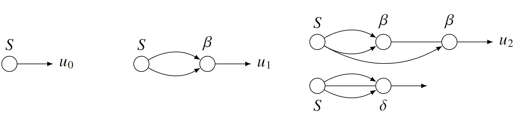
Pictorial description of Green function methord. The displacement is the sum of terms $u = u_{0} + u_{1} + u_{2} + \cdots$, where $u_{0}$ is the linear component of the displacement given by a Green function propagating a source. The first-order nonlinear term $u_{1}$ is given by the Green function propagating two waves from the source that interact with strength $\beta$. The Green function then propagates the result of the interaction. The second-order nonlinear term $u_{2}$ (for a compressional source) has two terms resulting from the Green function propagating three waves:(1) all three interact with strength $\delta$; or (2) two interact with strength $\beta$, propagate, and interact with the third with strength $\beta$. In both cases the Green function propagates the result of the interaction to the point of observation $x$.
Green 函数方法的图解说明。位移是各项之和 $u = u_{0} + u_{1}+ u_{2}+ \cdots$,其中 $u_{0}$ 是位移的线性分量,由传播源的 Green 函数给出。一阶非线性项 $u_{1}$ 是由 Green 函数给出的,该函数传播来自源的两个波,这两个波的相互作用强度为 $\beta$。然后,Green 函数传播相互作用的结果。二阶非线性项 $u_{2}$(对于压缩源)有两个项,由传播三个波的 Green 函数产生:(1)所有三个波都以强度为 $\delta$ 的方式相互作用;或(2)两个波以强度为 $\beta$ 的方式相互作用、传播,并以强度为 $\beta$ 的方式与第三个波相互作用。在这两种情况下,Green 函数都会将相互作用的结果传播到观测点 $x$。
Specific Solution
Specific solutions to $\eqref{eq:19}$ depend on our choices of Green function and external source. We have chosen to study the same geometry(an infinite solid) and therefore to use the same Green function for all of the examples described in the next section. Nevertheless, the examples apply to a broad range of problems depending on the external source and the physical characteristics to be studied.
The solution to $\eqref{eq:18}$ for the Green function of an infinite medium is
$$ \begin{equation} g_{\iota}(x,x^{\prime},\omega) = \frac{i}{2A_{\iota}(\omega)\chi(\omega)}e^{iA_{\iota}(\omega)|x-x^{\prime}|},\quad \iota = L,T, \tag{21}\label{eq:21} \end{equation} $$
where
$$ \begin{align} A_{\iota}(\omega) &= \kappa_{\iota}(\omega) + i\alpha_{\iota}(\omega),\tag{22a}\label{eq:22a}\\ \kappa_{\iota}(\omega) &= k_{\iota}\sqrt{\frac{r+s}{2[(1-\Delta)^{2} + |\omega\tau|^{2\nu}]}},\tag{22b}\label{eq:22b}\\ \alpha_{\iota}(\omega) &= k_{\iota}\sqrt{\frac{r-s}{2[(1-\Delta)^{2} + |\omega\tau|^{2\nu}]}},\tag{22c}\label{eq:22c}\\ r &= \sqrt{s^{2} + |\omega\tau|^{2\nu}\Delta^{2}},\tag{22d}\label{eq:22d}\\ s &= (1 - \Delta) + |\omega\tau|^{2\nu}. \tag{22e}\label{eq:22e} \end{align} $$
$\eqref{eq:19}$ 的具体解取决于我们对 Green 函数和外部源的选择。我们选择研究相同的几何形状(无限实体),因此在下一节描述的所有示例中使用相同的 Green 函数。不过,这些示例适用于多种问题,具体取决于外部源和要研究的物理特性。
对于无限介质的 Green 函数,$\eqref{eq:18}$ 的解是
$$ \begin{equation} g_{\iota}(x,x^{\prime},\omega) = \frac{i}{2A_{\iota}(\omega)\chi(\omega)}e^{iA_{\iota}(\omega)|x-x^{\prime}|},\quad \iota = L,T, \end{equation} $$
其中
$$ \begin{align} A_{\iota}(\omega) &= \kappa_{\iota}(\omega) + i\alpha_{\iota}(\omega),\tag{22a}\\ \kappa_{\iota}(\omega) &= k_{\iota}\sqrt{\frac{r+s}{2[(1-\Delta)^{2} + |\omega\tau|^{2\nu}]}},\tag{22b}\\ \alpha_{\iota}(\omega) &= k_{\iota}\sqrt{\frac{r-s}{2[(1-\Delta)^{2} + |\omega\tau|^{2\nu}]}},\tag{22c}\\ r &= \sqrt{s^{2} + |\omega\tau|^{2\nu}\Delta^{2}},\tag{22d}\\ s &= (1 - \Delta) + |\omega\tau|^{2\nu}. \tag{22e} \end{align} $$
The function, $\kappa_{\iota}$ and $\alpha_{\iota}(\omega)$, $\eqref{eq:22b}$ and $\eqref{eq:22c}$, define the dispersion relation and the attenuationin the system. If $\Delta=0$, then $\kappa_{\iota} = k_{\iota}$, $\alpha_{\iota}=0$ and we recover the Green function for propagation in an infinite medium in the absence of attenuation. The following asymptotic expression for $\kappa_{\iota}(\omega)$ and $\alpha_{\iota}(\omega)$ can be derived:
$$ \begin{align} &\kappa_{\iota}/k_{\iota}\rightarrow 1/\sqrt{1-\Delta}, &|\omega\tau|\ll 1,\\ &\kappa_{\iota}/k_{\iota}\rightarrow 1, &|\omega\tau|\gg 1,\\ &\alpha_{\iota}/|k_{\iota}|\rightarrow |\omega\tau|^{ \nu}\Delta/2(1-\Delta)^{3/2}, &|\omega\tau|\ll 1,\\ &\alpha_{\iota}/|k_{\iota}|\rightarrow |\omega\tau|^{-\nu}\Delta/2, &|\omega\tau|\gg 1. \end{align}\tag{23}\label{eq:23} $$
As we pass from $|\omega\tau|\ll 1$ through $|\omega\tau|=1$ to $|\omega\tau|\gg 1$, the normalized wave vector changes from one constant value to a lower constant value, while the normalized attenuation change from an $|\omega|^{\nu}$ dependence to an $|\omega|^{-\nu}$ dependence.
函数 $\kappa_{\iota}$ 和 $\alpha_{\iota}(\omega)$, $\eqref{eq:22b}$ 和 $\eqref{eq:22c}$ 定义了系统中的色散关系和衰减。如果 $\Delta=0$ ,那么 $\kappa_{\iota} = k_{\iota}$, $\alpha_{\iota}=0$,我们就恢复了在无衰减的无限介质中传播的 Green 函数。下面是 $\kappa_{\iota}(\omega)$ 和 $\alpha_{\iota}(\omega)$ 的渐近表达式:
$$ \begin{align} &\kappa_{\iota}/k_{\iota}\rightarrow 1/\sqrt{1-\Delta}, &|\omega\tau|\ll 1,\\ &\kappa_{\iota}/k_{\iota}\rightarrow 1, &|\omega\tau|\gg 1,\\ &\alpha_{\iota}/|k_{\iota}|\rightarrow |\omega\tau|^{ \nu}\Delta/2(1-\Delta)^{3/2}, &|\omega\tau|\ll 1,\\ &\alpha_{\iota}/|k_{\iota}|\rightarrow |\omega\tau|^{-\nu}\Delta/2, &|\omega\tau|\gg 1. \end{align}\tag{23} $$
当我们从 $|\omega\tau|\ll 1$ 经过 $|\omega\tau|=1$ 到 $|\omega\tau|\gg 1$ 时,归一化波矢量从一个常值变为一个较低的常值,而归一化衰减从 $|\omega|^{\nu}$ 依赖关系变为 $|\omega|^{-\nu}$ 依赖关系。
Given the Green functionin $\eqref{eq:21}$ and the source functions in $\eqref{eq:16a}$-$\eqref{eq:16f}$, the solution for the displacement field begins with the terms involving the external source $f_{i}^{(0)}(x,\omega)$. Since the $y$ and $z$ directions are identical by symmetry we choose $f_{z}^{(0)}(x,\omega) = 0$ and write $f_{x}^{(0)}(x,\omega)$ and $f_{y}^{(0)}(x,\omega)$ as source at the origin of the form
$$ \begin{align} f_{x}^{(0)}(x,\omega) &= -2i\chi(\omega)A_{L}(\omega)U_{L}\delta(x)F(\omega),\tag{24a}\label{eq:24a}\\ f_{y}^{(0)}(x,\omega) &= -2i\chi(\omega)A_{T}(\omega)U_{T}\delta(x)F(\omega),\tag{24b}\label{eq:24b} \end{align} $$
where $U_{L}$ and $U_{T}$ are the longitudinal and transverse displacement fields produced at the origin by the source, and $F(\omega)$ is the frequency spectrum of the source with units of time. Substituting $f_{i}^{(0)}(x,\omega)$ into $\eqref{eq:19}$, we find that the linear components of the displacement are
$$ \begin{align} u_{x}^{(0)}(x,\omega) &= U_{L}e^{iA_{L}(\omega)|x|}F(\omega),\tag{25a}\label{eq:25a}\\ u_{y}^{(0)}(x,\omega) &= U_{T}e^{iA_{T}(\omega)|x|}F(\omega),\tag{25b}\label{eq:25b}\\ u_{z}^{(0)}(x,\omega) &= 0. \tag{25c}\label{eq:25c} \end{align} $$
给定 $\eqref{eq:21}$ 中的 Green 函数和 $\eqref{eq:16a}$-$\eqref{eq:16f}$ 中的源函数,位移场的求解从涉及外部源的项 $f_{i}^{(0)}(x,\omega)$ 开始。由于 $y$ 和 $z$ 方向的对称性相同,我们选择 $f_{z}^{(0)}(x,\omega) = 0$,并将 $f_{x}^{(0)}(x,\omega)$ 和 $f_{y}^{(0)}(x,\omega)$ 写成原点处的源,其形式为
$$ \begin{align} f_{x}^{(0)}(x,\omega) &= -2i\chi(\omega)A_{L}(\omega)U_{L}\delta(x)F(\omega),\tag{24a}\\ f_{y}^{(0)}(x,\omega) &= -2i\chi(\omega)A_{T}(\omega)U_{T}\delta(x)F(\omega),\tag{24b} \end{align} $$
其中,$U_{L}$ 和 $U_{T}$ 是源在原点产生的纵向和横向位移场,$F(\omega)$ 是以时间为单位的源频谱。将 $f_{i}^{(0)}(x,\omega)$ 代入 $\eqref{eq:19}$,我们发现位移的线性分量为
$$ \begin{align} u_{x}^{(0)}(x,\omega) &= U_{L}e^{iA_{L}(\omega)|x|}F(\omega),\tag{25a}\\ u_{y}^{(0)}(x,\omega) &= U_{T}e^{iA_{T}(\omega)|x|}F(\omega),\tag{25b}\\ u_{z}^{(0)}(x,\omega) &= 0. \tag{25c} \end{align} $$
The source function $f_{i}^{(1)}$, $\eqref{eq:16b}$ and $\eqref{eq:16e}$, or the first-order nonlinear displacement terms are determined by the linear displacement terms in $\eqref{eq:25a}$-$\eqref{eq:25c}$. These first-order source functions yield first-order nonlinear displacementsof the form
$$ \begin{align} u_{x}^{(1)}(x,\omega) &= \beta U_{L}^{2}xE_{LL}(x,\omega) + \gamma U_{T}^{2}xE_{TT}(x,\omega),\tag{26a}\label{eq:26a}\\ u_{y}^{(1)}(x,\omega) &= \gamma U_{L}U_{T}x\frac{2c_{L}^{2}}{c_{T}^{2}}E_{LT}(x,\omega),\tag{26b}\label{eq:26b}\\ u_{z}^{(1)}(x,\omega) &= 0, \tag{26c}\label{eq:26c} \end{align} $$
where
$$ \begin{align} E_{LL}(x,\omega) &= \int\frac{\mathrm{d}\omega^{\prime}}{2\pi}\frac{e^{i[A_{L}(\omega^{\prime} + A_{L}(\phi))]|x|} - e^{iA_{L}(\omega)|x|}}{i[A_{L}(\omega^{\prime}) + A_{L}(\phi)- A_{L}(\omega)]|x|}C_{LL}(\omega,\omega^{\prime})F(\omega^{\prime})F(\phi),\tag{27a}\label{eq:27a}\\ E_{TT}(x,\omega) &= \int\frac{\mathrm{d}\omega^{\prime}}{2\pi}\frac{e^{i[A_{T}(\omega^{\prime}) + A_{T}(\phi)]|x|} - e^{iA_{L}(\omega)|x|}}{i[A_{T}(\omega^{\prime}) + A_{T}(\phi) - A_{L}(\omega)]|x|}C_{TT}(\omega,\omega^{\prime})F(\omega^{\prime})F(\phi),\tag{27b}\label{eq:27b}\\ E_{LT}(x,\omega) &= \int\frac{\mathrm{d}\omega^{\prime}}{2\pi}\frac{e^{i[A_{L}(\omega^{\prime}) + A_{T}(\phi)]|x|} - e^{iA_{T}(\omega)|x|}}{i[A_{L}(\omega^{\prime}) + A_{T}(\phi) - A_{T}(\omega)]|x|}C_{LT}(\omega,\omega^{\prime})F(\omega^{\prime})F(\phi),\tag{27c}\label{eq:27c} \end{align} $$
and
$$ \begin{align} C_{LL}(\omega,\omega^{\prime}) &= \frac{A_{L}(\omega^{\prime})A_{L}(\phi)[A_{L}(\omega^{\prime}) + A_{L}(\phi)]}{A_{L}(\omega^{\prime}) + A_{L}(\phi) + A_{L}(\omega)}\frac{\chi(\omega^{\prime})\chi(\phi)}{\chi(\omega)},\tag{28a}\label{eq:28a}\\ C_{TT}(\omega,\omega^{\prime}) &= \frac{A_{T}(\omega^{\prime})A_{T}(\phi)[A_{T}(\omega^{\prime}) + A_{T}(\phi)]}{A_{T}(\omega^{\prime}) + A_{T}(\phi) + A_{T}(\omega)}\frac{\chi(\omega^{\prime})\chi(\phi)}{\chi(\omega)},\tag{28b}\label{eq:28b}\\ C_{LT}(\omega,\omega^{\prime}) &= \frac{A_{L}(\omega^{\prime})A_{T}(\phi)[A_{L}(\omega^{\prime}) + A_{T}(\phi)]}{A_{L}(\omega^{\prime}) + A_{T}(\phi) + A_{T}(\omega)}\frac{\chi(\omega^{\prime})\chi(\phi)}{\chi(\omega)}. \tag{28c}\label{eq:28c} \end{align} $$
The resultsin $\eqref{eq:26a}$ and $\eqref{eq:26b}$ are arranged in the form of the product of an amplitude with a frequency- dependent envelope function. For example, the amplitude proportional to $\gamma$ in $\eqref{eq:26a}$ is proportional to $U_{T}^{2}$, as it is due to two transverse waves launched by the transverse source, and proportional to $x$, as the internal source works at all points between the point of observation and the external source point $x = 0$. The other amplitude factors can be understood in the same way. The envelope functions $E(x,\omega)$ describe the decay of the amplitude due to attenuation. For example, $E_{TT}(x,\omega)$ in $\eqref{eq:26a}$ contains the degradation of the strength of the internal source due to attenuation of the transverse displacement fields causing the source(the factor $\text{exp}\{-[\alpha_{T}(\omega^{\prime}) + \alpha_{T}(\phi)]|x|\}$) and attenuation of the displacement field between the internal source point and the point of detection (the factor $\text{exp}-\alpha_{L}(\omega)|x|$).
源函数 $f_{i}^{(1)}$、 $\eqref{eq:16b}$ 和 $\eqref{eq:16e}$ 或一阶非线性位移项是由 $\eqref{eq:25a}$-$\eqref{eq:25c}$ 中的线性位移项决定的。这些一阶源函数产生的一阶非线性位移形式为
$$ \begin{align} u_{x}^{(1)}(x,\omega) &= \beta U_{L}^{2}xE_{LL}(x,\omega) + \gamma U_{T}^{2}xE_{TT}(x,\omega),\tag{26a}\\ u_{y}^{(1)}(x,\omega) &= \gamma U_{L}U_{T}x\frac{2c_{L}^{2}}{c_{T}^{2}}E_{LT}(x,\omega),\tag{26b}\\ u_{z}^{(1)}(x,\omega) &= 0, \tag{26c} \end{align} $$
其中
$$ \begin{align} E_{LL}(x,\omega) &= \int\frac{\mathrm{d}\omega^{\prime}}{2\pi}\frac{e^{i[A_{L}(\omega^{\prime} + A_{L}(\phi))]|x|} - e^{iA_{L}(\omega)|x|}}{i[A_{L}(\omega^{\prime}) + A_{L}(\phi)- A_{L}(\omega)]|x|}C_{LL}(\omega,\omega^{\prime})F(\omega^{\prime})F(\phi),\tag{27a}\\ E_{TT}(x,\omega) &= \int\frac{\mathrm{d}\omega^{\prime}}{2\pi}\frac{e^{i[A_{T}(\omega^{\prime}) + A_{T}(\phi)]|x|} - e^{iA_{L}(\omega)|x|}}{i[A_{T}(\omega^{\prime}) + A_{T}(\phi) - A_{L}(\omega)]|x|}C_{TT}(\omega,\omega^{\prime})F(\omega^{\prime})F(\phi),\tag{27b}\\ E_{LT}(x,\omega) &= \int\frac{\mathrm{d}\omega^{\prime}}{2\pi}\frac{e^{i[A_{L}(\omega^{\prime}) + A_{T}(\phi)]|x|} - e^{iA_{T}(\omega)|x|}}{i[A_{L}(\omega^{\prime}) + A_{T}(\phi) - A_{T}(\omega)]|x|}C_{LT}(\omega,\omega^{\prime})F(\omega^{\prime})F(\phi),\tag{27c} \end{align} $$
和
$$ \begin{align} C_{LL}(\omega,\omega^{\prime}) &= \frac{A_{L}(\omega^{\prime})A_{L}(\phi)[A_{L}(\omega^{\prime}) + A_{L}(\phi)]}{A_{L}(\omega^{\prime}) + A_{L}(\phi) + A_{L}(\omega)}\frac{\chi(\omega^{\prime})\chi(\phi)}{\chi(\omega)},\tag{28a}\\ C_{TT}(\omega,\omega^{\prime}) &= \frac{A_{T}(\omega^{\prime})A_{T}(\phi)[A_{T}(\omega^{\prime}) + A_{T}(\phi)]}{A_{T}(\omega^{\prime}) + A_{T}(\phi) + A_{T}(\omega)}\frac{\chi(\omega^{\prime})\chi(\phi)}{\chi(\omega)},\tag{28b}\\ C_{LT}(\omega,\omega^{\prime}) &= \frac{A_{L}(\omega^{\prime})A_{T}(\phi)[A_{L}(\omega^{\prime}) + A_{T}(\phi)]}{A_{L}(\omega^{\prime}) + A_{T}(\phi) + A_{T}(\omega)}\frac{\chi(\omega^{\prime})\chi(\phi)}{\chi(\omega)}. \tag{28c} \end{align} $$
在 $\eqref{eq:26a}$ 和 $\eqref{eq:26b}$ 中的结果是以振幅与频率相关包络函数的乘积形式排列的。例如,$\eqref{eq:26a}$ 中与 $\gamma$ 成比例的振幅与 $U_{T}^{2}$ 成比例,因为它是由横向源发射的两个横波引起的,并且与 $x$ 成比例,因为内部源作用于观测点与外部源点 $x = 0$ 之间的所有点。其他振幅因子也可以用同样的方法来理解。 包络函数 $E(x,\omega)$ 描述了衰减引起的振幅衰减。例如,$\eqref{eq:26a}$ 中的 $E_{TT}(x,\omega)$ 包含了由于横向位移场衰减导致的内源强度衰减(因子 $\text{exp}\{-[\alpha_{T}(\omega^{\prime})+\alpha_{T}(\phi)]|x|\}$)和内部源点与探测点之间位移场的衰减(系数 $\text{exp}-\alpha_{L}(\omega)|x|$)。
In the limit of no attenuation, that is, $\chi(\omega)\equiv 1$, the envelope functions become
$$ \begin{align} E_{LL}(x,\omega) &= \int\frac{\mathrm{d}\omega^{\prime}}{2\pi}\frac{k_{L}^{\prime}(k_{L} - k_{L}^{\prime})}{2}F(\omega^{\prime})F(\phi)e^{ik_{L}|x|},\tag{29a}\label{eq:29a}\\ E_{TT}(x,\omega) &= \int\frac{\mathrm{d}\omega^{\prime}}{2\pi}\frac{k_{T}^{\prime}k_{T}(k_{T}-k_{T}^{\prime})}{i(k_{T}^{2} - k_{L}^{2})|x|}F(\omega^{\prime})F(\phi)\left(e^{ik_{T}|x|} - e^{ik_{L}|x|}\right),\tag{29b}\label{eq:29b}\\ E_{LT}(x,\omega) &= \int\frac{\mathrm{d}\omega^{\prime}}{2\pi}\frac{k_{L}^{\prime}(k_{T} - k_{T}^{\prime})(k_{L}^{\prime} + k_{T} - k_{T}^{\prime})}{i(k_{L}^{\prime} -k_{T}^{\prime} + 2k_{T})(k_{L}^{\prime} - k_{T}^{\prime})|x|}F(\omega^{\prime})F(\phi)\left( e^{i(k_{L}^{\prime} + k_{T} - k_{T}^{\prime})} - e^{ik_{T}|x|}\right),\tag{29c}\label{eq:29c} \end{align} $$
where $k^{\prime} = \omega^{\prime}/c$. Note that the linear $x$ dependence of the amplitudes in $\eqref{eq:26a}$ and $\eqref{eq:26b}$ will cancel with the $x$ dependence of the envelope functions in all but the longitudinal-longitudinal wave interaction($E_{LL}$).
在没有衰减的情况下,即 $\chi(\omega)\equiv 1$,包络函数变为
$$ \begin{align} E_{LL}(x,\omega) &= \int\frac{\mathrm{d}\omega^{\prime}}{2\pi}\frac{k_{L}^{\prime}(k_{L} - k_{L}^{\prime})}{2}F(\omega^{\prime})F(\phi)e^{ik_{L}|x|},\tag{29a}\\ E_{TT}(x,\omega) &= \int\frac{\mathrm{d}\omega^{\prime}}{2\pi}\frac{k_{T}^{\prime}k_{T}(k_{T}-k_{T}^{\prime})}{i(k_{T}^{2} - k_{L}^{2})|x|}F(\omega^{\prime})F(\phi)\left(e^{ik_{T}|x|} - e^{ik_{L}|x|}\right),\tag{29b}\\ E_{LT}(x,\omega) &= \int\frac{\mathrm{d}\omega^{\prime}}{2\pi}\frac{k_{L}^{\prime}(k_{T} - k_{T}^{\prime})(k_{L}^{\prime} + k_{T} - k_{T}^{\prime})}{i(k_{L}^{\prime} -k_{T}^{\prime} + 2k_{T})(k_{L}^{\prime} - k_{T}^{\prime})|x|}F(\omega^{\prime})F(\phi)\left( e^{i(k_{L}^{\prime} + k_{T} - k_{T}^{\prime})} - e^{ik_{T}|x|}\right),\tag{29c} \end{align} $$
其中 $k^{\prime} = \omega^{\prime}/c$。请注意,除了纵波-纵波相互作用($E_{LL}$)之外,$\eqref{eq:26a}$ 和 $\eqref{eq:26b}$ 中振幅的线性 $x$ 依赖性将与包络函数的 $x$ 依赖性相抵消。
Examples
Continuous Single-Frequency Sine Wave
As the first example we choose the external driving force to be a continuous single-frequency compressional sine wave at the origin with displacement amplitude $U$. That is, in $\eqref{eq:24a}$ and $\eqref{eq:24b}$, let $U_{L} = U$, $U_{T} = 0$, and
$$ \begin{equation} F(\omega) = 2\pi\frac{1}{2i}[\delta(\omega - \omega_{0}) - \delta(\omega + \omega_{0})]. \tag{30}\label{eq:30} \end{equation} $$
Displacement occurs only in the $x$ direction.
From $\eqref{eq:25a}$ and $\eqref{eq:7a}$, the linear displacement is
$$ \begin{equation} u_{x}^{(0)}(x,t) = \frac{U}{2i}\left[e^{i[A_{L}(\omega_{0})|x| - \omega_{0}t]} - e^{i[A_{L}(-\omega_{0})|x| + \omega_{0}t]}\right]. \tag{31a}\label{eq:31a} \end{equation} $$
Equation $\eqref{eq:31a}$ reduces to a sine wave modified by an exponentially decaying envelope in both the high- and low-frequency limits:
$$ u_{x}^{(0)}(x,t) \rightarrow Ue^{-\alpha_{m}|x|}\sin{(k_{m}|x|-\omega_{0}t)},\tag{31b}\label{eq:31b} $$
where
$$ \begin{align} k_{m} &= k_{P} = \omega_{0} / c_{L}\sqrt{1-\Delta}, &|\omega\tau|\ll 1,\\ k_{m} &= k_{0} = \omega_{0} / c_{L}, &|\omega\tau|\gg 1,\\ \alpha_{m} &= \alpha_{P} = k_{P}(\omega_{0}\tau)^{\nu}\Delta/2(1-\Delta), &|\omega\tau|\ll 1,\\ \alpha_{m} &= \alpha_{H} = k_{0}(\omega_{0}\tau)^{-\nu}\Delta/2, &|\omega\tau|\gg 1. \end{align}\tag{32}\label{eq:32} $$
作为第一个例子,我们选择外部驱动力为原点处位移振幅为 $U$ 的连续单频正弦压缩波。也就是说,在 $\eqref{eq:24a}$ 和 $\eqref{eq:24b}$ 中,设 $U_{L} = U$,$U_{T} = 0$,并且
$$ \begin{equation} F(\omega) = 2\pi\frac{1}{2i}[\delta(\omega - \omega_{0}) - \delta(\omega + \omega_{0})]. \tag{30} \end{equation} $$
位移只发生在 $x$ 方向。根据 $\eqref{eq:25a}$ 和 $\eqref{eq:7a}$,线性位移为
$$ \begin{equation} u_{x}^{(0)}(x,t) = \frac{U}{2i}\left[e^{i[A_{L}(\omega_{0})|x| - \omega_{0}t]} - e^{i[A_{L}(-\omega_{0})|x| + \omega_{0}t]}\right]. \tag{31a} \end{equation} $$
方程 $\eqref{eq:31a}$ 在高频和低频范围内都被指数衰减包络修饰成正弦波:
$$ u_{x}^{(0)}(x,t) \rightarrow Ue^{-\alpha_{m}|x|}\sin{(k_{m}|x|-\omega_{0}t)},\tag{31b} $$
其中
$$ \begin{align} k_{m} &= k_{P} = \omega_{0} / c_{L}\sqrt{1-\Delta}, &|\omega\tau|\ll 1,\\ k_{m} &= k_{0} = \omega_{0} / c_{L}, &|\omega\tau|\gg 1,\\ \alpha_{m} &= \alpha_{P} = k_{P}(\omega_{0}\tau)^{\nu}\Delta/2(1-\Delta), &|\omega\tau|\ll 1,\\ \alpha_{m} &= \alpha_{H} = k_{0}(\omega_{0}\tau)^{-\nu}\Delta/2, &|\omega\tau|\gg 1. \end{align}\tag{32} $$
From $\eqref{eq:26a}$ and $\eqref{eq:7a}$, the first-order nonlinear displacement is
$$ \begin{align} u_{x}^{(1)} = -\frac{\beta U^{2}x}{4}\left[\frac{|\chi(\omega_{0})A_{L}(\omega_{0})|^{2}}{\chi(0)}\frac{1-e^{-2\alpha_{L}(\omega_{0})|x|}}{2\alpha_{L}(\omega_{0})|x|} + \frac{4}{|x|}\text{Im}\left\{\frac{\chi^{2}(\omega_{0})A_{L}^{3}(\omega_{0})}{\chi(2\omega_{0})} \frac{e^{i2A_{L}(\omega_{0})|x|} - e^{iA_{L}(2\omega_{0})|x|}}{4A_{L}^{2}(\omega_{0}) - A_{L}^{2}(2\omega_{0})}\right\}\right]. \tag{33a}\label{eq:33a} \end{align} $$
At low and high frequencie, $\eqref{eq:33a}$ reduces to the sum of a cosine at $2\omega_{0}$ and a zero frequency term. Both terms are modified by attenuative exponentials. In the limit $\omega_{0}\tau\ll 1$,
$$ \begin{align} u_{x}^{(1)}\rightarrow -\frac{\beta U^{2}k_{0}^{2}x}{4}\left[\frac{1 - e^{-2\alpha_{P}|x|}}{2\alpha_{P}|x|} + \frac{e^{-2\alpha_{P}|x|} - e^{-2^{1+\nu}\alpha_{P}|x|}}{2(2^{\nu} - 1)\alpha_{P}|x|}\cos{(2k_{P}|x|-2\omega_{0}t)}\right],\tag{33b}\label{eq:33b} \end{align} $$
in agreemenwt ith the results of Polyakova[1964]. In the limit $\omega_{0}\tau\gg 1$,
$$ \begin{equation} u_{x}^{(1)}(x,t)\rightarrow -\frac{\beta U^{2}k_{0}^{2}x}{4}\left[\frac{1 - e^{-2\alpha_{P}|x|}}{2(1-\Delta)\alpha_{P}|x|} + \frac{e^{-2^{1-\nu}\alpha_{P}|x|} - e^{-2\alpha_{P}|x|}}{2(1-2^{-\nu})\alpha_{P}|x|}\cos{(2k_{0}|x| - 2\omega_{0}t)}\right]. \tag{33c}\label{eq:33c} \end{equation} $$
根据 $\eqref{eq:26a}$ 和 $\eqref{eq:7a}$,一阶非线性位移为
$$ \begin{align} u_{x}^{(1)} = -\frac{\beta U^{2}x}{4}\left[\frac{|\chi(\omega_{0})A_{L}(\omega_{0})|^{2}}{\chi(0)}\frac{1-e^{-2\alpha_{L}(\omega_{0})|x|}}{2\alpha_{L}(\omega_{0})|x|} + \frac{4}{|x|}\text{Im}\left\{\frac{\chi^{2}(\omega_{0})A_{L}^{3}(\omega_{0})}{\chi(2\omega_{0})} \frac{e^{i2A_{L}(\omega_{0})|x|} - e^{iA_{L}(2\omega_{0})|x|}}{4A_{L}^{2}(\omega_{0}) - A_{L}^{2}(2\omega_{0})}\right\}\right]. \tag{33a} \end{align} $$
在低频和高频下,$\eqref{eq:33a}$ 约为在 $2\omega_{0}$ 处的余弦项和一个零频率项的总和。这两个项都由衰减指数修正。在 $\omega_{0}\tau\ll 1$ 极限下,
$$ \begin{align} u_{x}^{(1)}\rightarrow -\frac{\beta U^{2}k_{0}^{2}x}{4}\left[\frac{1 - e^{-2\alpha_{P}|x|}}{2\alpha_{P}|x|} + \frac{e^{-2\alpha_{P}|x|} - e^{-2^{1+\nu}\alpha_{P}|x|}}{2(2^{\nu} - 1)\alpha_{P}|x|}\cos{(2k_{P}|x|-2\omega_{0}t)}\right],\tag{33b} \end{align} $$
与 Polyakova [1964] 的结果一致。在 $\omega_{0}\tau\gg 1$ 极限下,
$$ \begin{equation} u_{x}^{(1)}(x,t)\rightarrow -\frac{\beta U^{2}k_{0}^{2}x}{4}\left[\frac{1 - e^{-2\alpha_{P}|x|}}{2(1-\Delta)\alpha_{P}|x|} + \frac{e^{-2^{1-\nu}\alpha_{P}|x|} - e^{-2\alpha_{P}|x|}}{2(1-2^{-\nu})\alpha_{P}|x|}\cos{(2k_{0}|x| - 2\omega_{0}t)}\right]. \tag{33c} \end{equation} $$
In Figure 2, we show the transition of the first-order nonlinear term from $\omega_{0}\tau\ll 1$ to $\omega_{0}\tau\gg 1$ at three distances from the source. The normalized $u_{x}^{(1)}(x,t)$ values from $\eqref{eq:33a}$, $\eqref{eq:33b}$, and $\eqref{eq:33c}$ are shown as a function of $\omega_{0}\tau$ for a source frequency of $10\text{ Hz}$. The parameter values are $c = 6000\text{ m/s}$; $\Delta = 0.2$; $\nu = 1$; and $x = 0.6$, $6$, and $60\text{ km}$. Since the source is continuous, we chose $t = 0$. The dashed curves in Figure 2 are the $\omega_{0}\tau\ll 1$ results; the dotted curves are the $\omega_{0}\tau\gg 1$ results.
在图 2 中,我们展示了一阶非线性项在距离源的三个距离上从 $\omega_{0}\tau\ll 1$ 到 $\omega_{0}\tau\gg 1$ 的转变。来自 $\eqref{eq:33a}$、$\eqref{eq:33b}$ 和 $\eqref{eq:33c}$ 的归一化 $u_{x}^{(1)}(x,t)$ 值显示为源频率为 $10\text{ Hz}$ 时 $\omega_{0}\tau$ 的函数。参数值为:$c = 6000\text{ m/s}$; $\Delta = 0.2$; $\nu = 1$; $x = 0.6$, $6$, 和 $60\text{ km}$。由于源是连续的,我们选择了 $t = 0$。图 2 中的虚线是 $\omega_{0}\tau\ll 1$ 的结果;虚线是 $\omega_{0}\tau\gg 1$ 的结果。
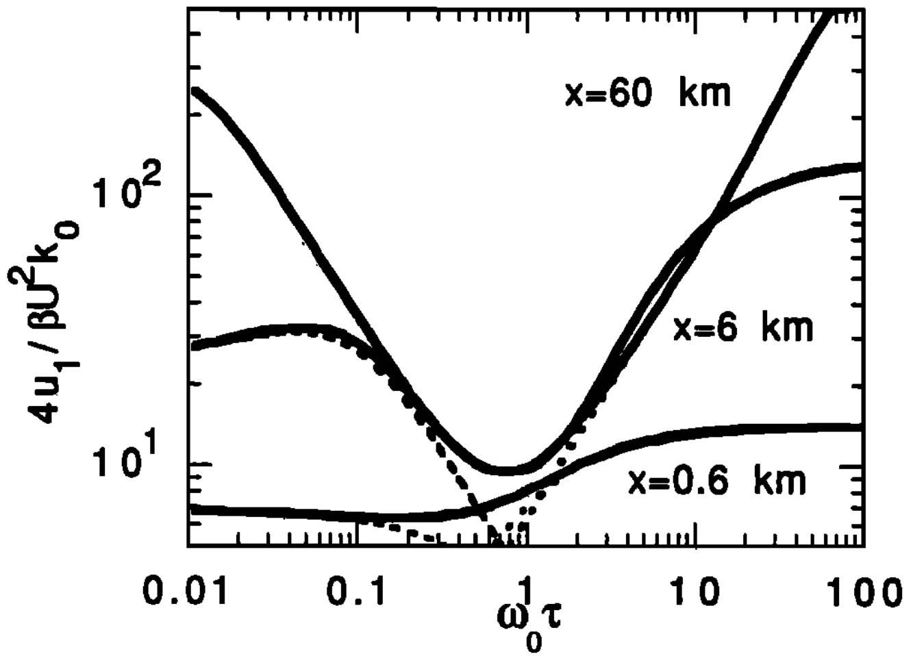
Attenuation dependence of the first-order nonlinear displacement. The normalized first-order nonlinear displacementis shown as a function of $\omega_{0}\tau$. The solid curves are calculated from $\eqref{eq:33a}$ at distances $x = 0.6$, $6$, and $60\text{ km}$. The source frequency is $10\text{ Hz}$, $\Delta = 0.2$, and $\nu = 1$. The value of $\tau$ is varied. The dashed curves are the low $\omega_{0}\tau$ limit, $\eqref{eq:33b}$; the dotted curves are the high $\omega_{0}\tau$ limit, $\eqref{eq:33c}$. The crossover from low to high $\omega_{0}\tau$ and the point of maximum attenuation are at $\omega_{0}\tau\approx 1$.
一阶非线性位移的衰减依赖性。归一化的一阶非线性位移是 $\omega_{0}\tau$ 的函数。实心曲线是在距离 $x=0.6$、$6$ 和 $60\text{ km}$ 时根据 $\eqref{eq:33a}$ 计算得出的。源频率为 $10\text{ Hz}$,$\Delta = 0.2$,$\nu = 1$。$\tau$ 的值是变化的。虚线为低 $\omega_{0}\tau$ 限值,即 $\eqref{eq:33b}$;虚线为高 $\omega_{0}\tau$ 限值,即 $\eqref{eq:33c}$。从低 $\omega_{0}\tau$ 到高 $\omega_{0}\tau$ 的交叉点和最大衰减点约为 $\omega_{0}\tau$。
In the absence of attenuation($\alpha x\ll 1$) we have the familiar result
$$ \begin{equation} u_{x}(x,t) = u_{x}^{(0)} + u_{x}^{(1)} = U\sin{(k_{0}|x|-\omega_{0}t)}-\frac{\beta U^{2}k_{0}^{2}x}{4}[1 + \cos{(2k_{0}|x| - 2\omega_{0}t)}], \tag{34}\label{eq:34} \end{equation} $$
to first order in the nonlinearity. Thus the displacement amplitude of the $2\omega_{0}$ harmonic grows as the square of the amplitude of the fundamental, the square of the frequency, linearly with distance, and linearly with the material parameter $\beta$.
For the case discussed here of displacement due to a compressional source in the $x$ direction, the equation of motion $\eqref{eq:6a}$ maybe easily expanded to include quartic anharmonicity as well as cubic anharmonicity:
$$ \begin{equation} \frac{1}{c_{L}^{2}}\ddot{u}_{x} = \frac{\partial}{\partial x}\left[\frac{\partial u_{x}}{\partial x} + \beta\left(\frac{\partial u_{x}}{\partial x}\right)^{2} + \delta\left(\frac{\partial u_{x}}{\partial x}\right)^{3}\right] + S_{x},\tag{35}\label{eq:35} \end{equation} $$
where $\beta$ and $\delta$ are measures of the strength of the cubic and quartic anharmonicity, respectively. Given the equation of motion in $\eqref{eq:35}$, the second-order source function $f_{x}^{(2)}$ becomes
$$ \begin{equation} f_{x}^{(2)}(x,\omega) = \frac{\partial }{\partial x}\int\frac{\mathrm{d}\omega^{\prime}}{2\pi}\chi(\omega^{\prime})\left[\delta\frac{\partial u_{x}^{(0)}(x,\omega^{\prime})}{\partial x}\int\frac{\mathrm{d}\omega^{\prime\prime}}{2\pi}\chi(\omega^{\prime\prime})\chi(\psi)\frac{\partial u_{x}^{(0)}(x,\omega^{\prime\prime})}{\partial x}\frac{\partial u_{x}^{(0)}(x,\psi)}{\partial x} + 2\beta\chi(\phi)\frac{\partial u_{x}^{(0)}(x,\omega^{\prime})}{\partial x}\frac{\partial u_{x}^{(1)}(x,\phi)}{\partial x}\right],\tag{36}\label{eq:36} \end{equation} $$
where $\psi = \omega - \omega^{\prime} - \omega^{\prime\prime}$. In the absence of attenuation, the source function $\eqref{eq:36}$ leads to a second-order nonlinear displacement:
$$ \begin{align} u_{x}^{(2)}(x,t) &= \frac{U^{3}k_{0}^{3}}{8}\left[(4\beta^{2} - 3\delta)|x|\cos{(k_{0}|x| - \omega_{0}t)}\right.\\ &\left.+\left(\frac{3\delta}{k_{0}} - \frac{4\beta^{2}}{k_{0}} - \beta^{2}k_{0}x^{2}\right)\sin{(k_{0}x - \omega_{0}t)}\right.\\ &\left.+\left(\frac{\delta}{3k_{0}} - \frac{4\beta^{2}}{9k_{0}} - \beta^{2}k_{0}x^{2}\right) \sin{(3k_{0}|x|-3\omega_{0}t)}\right.\\ &\left.\left(\frac{4\beta^{2}}{3} - \delta\right)|x|\cos{(3k_{0}|x| - 3\omega_{0}t)}\right]. \tag{37}\label{eq:37} \end{align} $$
The interactions producing the displacement of $\eqref{eq:37}$ are illustrated in Figure 1. The second-ordenr nonlinear displacement has components at $\omega_{0}$ and $3\omega_{0}$. The displacement amplitude grows as the cube of the amplitude of the fundamental and the cube of the frequency. At a large propagation distance, the displacement amplitude depends on the square of $\beta$ and the square of the propagation distance. Note that the quartic anharmonic coefficient $\delta$ must be of the order $\beta^{2}$ in order to make a significant contribution to the second order nonlinear displacement. From a literature study of velocity versus pressure data on a variety of rocktypes, this seems to be the case ($\delta\approx \beta^{2}$) (G. D. Meegan, Jr., unpublished data, 1993).
在没有衰减的情况下($\alpha x\ll 1$),我们会得到熟悉的结果
$$ \begin{equation} u_{x}(x,t) = u_{x}^{(0)} + u_{x}^{(1)} = U\sin{(k_{0}|x|-\omega_{0}t)}-\frac{\beta U^{2}k_{0}^{2}x}{4}[1 + \cos{(2k_{0}|x| - 2\omega_{0}t)}], \tag{34} \end{equation} $$
达到非线性的一阶。因此,$2\omega_{0}$ 谐波的位移振幅随着基波振幅的平方、频率的平方、距离的线性增长以及材料参数 $\beta$ 的线性增长而增长。
对于本文讨论的由 $x$ 方向上的压缩源引起的位移,运动方程 $\eqref{eq:6a}$ 可以很容易地扩展到包括四次谐波和三次谐波:
$$ \begin{equation} \frac{1}{c_{L}^{2}}\ddot{u}_{x} = \frac{\partial}{\partial x}\left[\frac{\partial u_{x}}{\partial x} + \beta\left(\frac{\partial u_{x}}{\partial x}\right)^{2} + \delta\left(\frac{\partial u_{x}}{\partial x}\right)^{3}\right] + S_{x},\tag{35} \end{equation} $$
其中,$\beta$ 和 $\delta$ 分别是三次谐波和四次谐波强度的度量。考虑到 $\eqref{eq:35}$ 中的运动方程,二阶源函数 $f_{x}^{(2)}$ 变为
$$ \begin{equation} f_{x}^{(2)}(x,\omega) = \frac{\partial }{\partial x}\int\frac{\mathrm{d}\omega^{\prime}}{2\pi}\chi(\omega^{\prime})\left[\delta\frac{\partial u_{x}^{(0)}(x,\omega^{\prime})}{\partial x}\int\frac{\mathrm{d}\omega^{\prime\prime}}{2\pi}\chi(\omega^{\prime\prime})\chi(\psi)\frac{\partial u_{x}^{(0)}(x,\omega^{\prime\prime})}{\partial x}\frac{\partial u_{x}^{(0)}(x,\psi)}{\partial x} + 2\beta\chi(\phi)\frac{\partial u_{x}^{(0)}(x,\omega^{\prime})}{\partial x}\frac{\partial u_{x}^{(1)}(x,\phi)}{\partial x}\right],\tag{36} \end{equation} $$
其中 $\psi = \omega - \omega^{\prime} - \omega^{\prime\prime}$. 在没有衰减的情况下,源函数 $\eqref{eq:36}$ 会导致二阶非线性位移:
$$ \begin{align} u_{x}^{(2)}(x,t) &= \frac{U^{3}k_{0}^{3}}{8}\left[(4\beta^{2} - 3\delta)|x|\cos{(k_{0}|x| - \omega_{0}t)}\right.\\ &\left.+\left(\frac{3\delta}{k_{0}} - \frac{4\beta^{2}}{k_{0}} - \beta^{2}k_{0}x^{2}\right)\sin{(k_{0}x - \omega_{0}t)}\right.\\ &\left.+\left(\frac{\delta}{3k_{0}} - \frac{4\beta^{2}}{9k_{0}} - \beta^{2}k_{0}x^{2}\right) \sin{(3k_{0}|x|-3\omega_{0}t)}\right.\\ &\left.\left(\frac{4\beta^{2}}{3} - \delta\right)|x|\cos{(3k_{0}|x| - 3\omega_{0}t)}\right]. \tag{37} \end{align} $$
产生 $\eqref{eq:37}$ 位移的相互作用如图 1 所示。二阶非线性位移在 $\omega_{0}$ 和 $3\omega_{0}$ 处有分量。位移振幅随着基频振幅的立方和频率的立方而增长。在传播距离较大时,位移振幅取决于 $\beta$ 的平方和传播距离的平方。需要注意的是,四元谐波系数 $\delta$ 必须达到 $\beta^{2}$ 的数量级,才能对二阶非线性位移做出显著贡献。根据对各种岩石类型的速度与应力数据的文献研究,情况似乎就是这样($\delta\approx \beta^{2}$)(G. D. Meegan, Jr., 未发表数据,1993 年)。
In Figure 3 we show the displacement amplitudes of each frequency component in $\eqref{eq:34}$ and $\eqref{eq:37}$. Figure 3a is a plot of the amplitude at the source frequency and the first two harmonics as a function of propagation distance. Figure 3b is a plot of the amplitude as a function of the source frequency. The first harmonic ($2f$) grows linearly with propagation distance and as the square of the source frequency; the second harmonic ($3f$) grows as the square of the propagation distance and as the fourth power of the source frequency. The parameters used in the calculation are $U=5\times 10^{-4}\text{ m}$ (corresponding to strains of order $10^{-6}$), $c_{L} = 6000\text{ m/s}$, $\beta = -10^{3}$ [Meegan et al., 1993], and $\delta = -10^{6}$. In Figure 3a the frequency $f$ is $3\text{ Hz}$, and in Figure 3b the propagation distance $x$ is $10\text{ km}$. Attenuation is not included.
图 3 显示了 $\eqref{eq:34}$ 和 $\eqref{eq:37}$ 中各频率分量的位移振幅。图 3a 是源频率和前两次谐波的振幅与传播距离的函数关系图。图 3b 是振幅与声源频率的函数关系图。第一次谐波($2f$)随传播距离线性增长,并随声源频率的平方而增长;第二次谐波($3f$)随传播距离的平方和声源频率的四次幂而增长。计算中使用的参数为:$U=5\times 10^{-4}\text{ m}$(对应于 $10^{-6}$ 数量级的应变),$c_{L} = 6000\text{ m/s}$,$\beta = -10^{3}$ [Meegan 等人,1993],以及 $\delta = -10^{6}$。图 3a 中的频率 $f$ 为 $3\text{ Hz}$,图 3b 中的传播距离 $x$ 为 $10\text{km}$。衰减不包括在内。
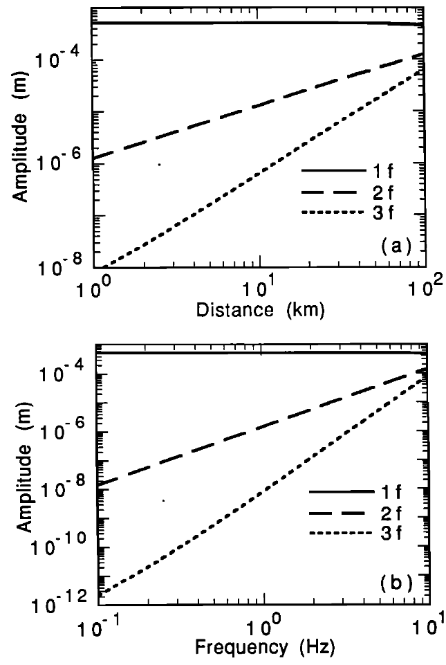
Displacement amplitudes for individual frequency components. Attenuation is not included. Solid curves are the amplitudes of the source frequency $1f$, long-dash curves are the amplitudes of the first harmonic $2f$, and short-dashcurves are the amplitudes of the second harmonic $3f$. (a) Displacement amplitude as a function of propagation distance. The $1f$ amplitude decreases slightly, the $2f$ amplitude increases linearly with distance, and the $3f$ amplitude increases quadratically with distance. (b) Displacement amplitude as a function of source frequency at $x=10\text{ km}$. The $1f$ amplitude decreases slightly, the $2f$ amplitude increases as the square of the frequency, and the $3f$ amplitude increases as the fourth power of the frequency.
各频率成分的位移幅度。不包括衰减。实线曲线为源频率 $1f$ 的振幅,长斜线曲线为一次谐波 $2f$ 的振幅,短斜线曲线为二次谐波 $3f$ 的振幅。 (a) 位移振幅与传播距离的函数关系。$1f$ 振幅略有减小,$2f$ 振幅随距离线性增加,$3f$ 振幅随距离二次增加。 (b) $x=10\text{ km}$ 处的位移振幅与源频率的函数关系。$1f$ 振幅略有减小,$2f$ 振幅随频率的平方而增大,$3f$ 振幅随频率的四次方而增大。
Broadband Source
A seismic source produces a broadband frequency spectrum. In order to explore whether nonlinear effects modify seismic spectra significantly, we chose $U_{L} = U$ and $U_{T} = 0$ in $\eqref{eq:24a}$ and $\eqref{eq:24b}$ and use
$$ \begin{equation} F(\omega) = \frac{\Omega}{(i\omega - \Omega)^{2}}, \tag{38a}\label{eq:38a} \end{equation} $$
as the external source[Yu et al., 1992]. The transform of $\eqref{eq:38a}$ is
$$ \begin{equation} F(t) = \Omega t e^{-\Omega t}. \tag{38b}\label{eq:38b} \end{equation} $$
As shown in Figure 4, this choice of external source is band limited in time and has a frequency spectrum that is flat for low frequencies and falls off as $\omega^{-2}$ for high frequencies.
地震源会产生宽带频谱。为了探索非线性效应是否会显著改变地震频谱,我们在 $\eqref{eq:24a}$ 和 $\eqref{eq:24b}$ 中选择了 $U_{L} = U$ 和 $U_{T} = 0$,并使用了
$$ \begin{equation} F(\omega) = \frac{\Omega}{(i\omega - \Omega)^{2}}, \tag{38a} \end{equation} $$
作为外部源[Yu 等人,1992]。$\eqref{eq:38a}$ 的变换是
$$ \begin{equation} F(t) = \Omega t e^{-\Omega t}. \tag{38b} \end{equation} $$
如图 4 所示,所选择的外部源在时间上有频带限制,其频谱在低频时平坦,在高频时下降为 $\omega^{-2}$。

Broadband source function. (a) Time domain, $\eqref{eq:38b}$, $\Omega = 40\text{ rad}$. (b) Frequency domain, $\eqref{eq:38a}$. This source function is time limited and has a frequency spectrum that is flat at low frequencies and falls off as $\omega^{-2}$ at high frequencies, thereby providing a useful idealization of a seismic source.
宽带源函数。(a) 时域,$\eqref{eq:38b}$, $\Omega = 40\text{ rad}$。(b) 频域,$\eqref{eq:38a}$。这个震源函数是有时间限制的,其频谱在低频时是平坦的,在高频时会随着 $\omega^{-2}$ 的下降而下降,从而提供了一个有用的理想化震源。
In Figure 5 we show the displacement field as a function of frequency resulting from a source producing the frequency spectrum of $\eqref{eq:38a}$. We calculated the received frequency spectrum at four distances from the source ($x = 1$, $10$, $20$, and $40\text{ km}$) with linear and first order nonlinear terms taken into account, $\eqref{eq:25a}$ and $\eqref{eq:26a}$. Figure 5a shows the evolution of the frequency spectrum in the absence of attenuation. Figure 5b shows the evolution of the frequency spectrum where $Q\approx 100$. We chose $\tau$, $\Delta$, and $\nu$ such that the model $Q$ is approximately equal to the measured $Q$ in central California [Mayeda et al., 1992]. The parameters used in the calculation are $\Omega = 40\text{ Hz}$, $U = 10^{-3}\text{ m}$ (corresponding to strains of order $10^{-6}$), $c_{L} = 6000\text{ m/s}$, $\beta = -10^{3}$ [Meegan et al., 1993], $\Delta = 0.05$, $\nu = 1$, and $\tau = 0.3\text{ s}$.
图 5 显示了产生 $\eqref{eq:38a}$ 频谱的声源所产生的位移场与频率的函数关系。我们计算了距离声源四个距离($x = 1$、$10$、$20$ 和 $40\text{ km}$)下的接收频谱,并考虑了线性和一阶非线性项,即 $\eqref{eq:25a}$ 和 $\eqref{eq:26a}$。图 5a 显示了没有衰减时频谱的演变。图 5b 显示了 $Q\approx 100$ 时的频谱变化。我们选择了 $\tau$、$\Delta$ 和 $\nu$,使模型中的 $Q$ 与加利福尼亚中部的实测 $Q$ 大致相等 [Mayeda 等人]. 计算中使用的参数为:$\Omega = 40\text{ Hz}$、$U = 10^{-3}\text{ m}$(对应于 $10^{-6}$ 级的应变)、$c_{L} = 6000\text{ m/s}$、$\beta = -10^{3}$ [Meegan 等人, 1993]、$\Delta = 0.05$、$\nu = 1$、$\tau = 0.3\text{ s}$。
Clearly, higher frequencies are being created in the nonlinear interaction as a function of propagation distance. Note especially the decrease in the roll-off slope and corner frequency in Figure 5b. The amplitudes of sum and difference frequency components depend on the competition between growth with propagation distance due to nonlinearity and decay with distance due to attenuation. These results are in qualitative agreement with the numerical results of Yu et al. [1992] in a study of nonlinear soil response which concluded that nonlinearity enhances high frequencies at the expense of intermediate frequencies.
显然,随着传播距离的增加,非线性相互作用产生了更高的频率。请特别注意图 5b 中滚降斜率和角频率的下降。和差频率分量的振幅取决于非线性随传播距离增长和衰减随传播距离而耗散之间的竞争。这些结果与 Yu 等人[1992]在非线性土壤响应研究中的数值结果在本质上是一致的,后者认为非线性增强了高频,但牺牲了中频。

Displacement frequency spectrum of a broadband source, $\eqref{eq:38a}$. The pulse propagates to $x = 1\text{ km}$, $10\text{ km}$, $20\text{ km}$, and $40\text{ km}$, progressively producing sum and difference frequencies through a first-order nonlinear interaction. (a) In the absence of attenuation; (b) including attenuation, $Q\approx 100$. The high- frequency contribution to the spectrum become smore pronounced as the wave propagates.
宽带信号源的位移频谱,$\eqref{eq:38a}$。脉冲传播到 $x=1\text{km}$、$10\text{km}$、$20\text{km}$ 和 $40\text{km}$,通过一阶非线性相互作用逐步产生和差频率。(a) 在无衰减的情况下;(b) 包括衰减,$Q\approx 100$。随着波的传播,频谱中的高频贡献变得更加明显。
Conclusions
In this paper we have developed and illustrated a theoretical framework for investigating the nonlinear interaction of frequency components in large-amplitude elastic waves. We derived the equation of motion for the displacement field to third order in the strain, including attenuation by allowing the displacement derivative to have both instantaneous and retarded components. We solved the equation of motion by using the exact Green function solution to the linear problem and developing higher-order displacement components in terms of the exact solution. This method has conceptual clarity and a high degree of flexibility. It is a good approximation to an exact solution in cases where the energy shift due to nonlinear terms in the displacement is small (less than $10\%$), a limit that applies to many geophysical applications.
本文为研究大振幅弹性波中频率成分的非线性相互作用建立了一个理论框架,并对其进行了说明。我们推导出了应变三阶位移场的运动方程,包括允许位移导数具有瞬时分量和延迟分量的衰减。我们通过使用线性问题的精确 Green 函数解来求解运动方程,并根据精确解建立高阶位移分量。这种方法概念清晰,灵活性高。在位移中非线性项引起的能量移动很小(小于 $10\%$)的情况下,它可以很好地近似于精确解,这种限制适用于许多地球物理应用。
We have illustrated the use of the Green function technique in two examples.
(1) We solved analytically for the displacement field produced by a continuous single-frequency sine wave source to first order in the nonlinearity including attenuation and to secondorder in the nonlinearity in the absence of attenuation. We found that the first-order term, with components at twice the source frequency and at zero frequency, grows linearly with propagation distance and nonlinear coefficient and as the square of the initial displacement and source frequency. Asymptotically, the second-order term grows as the square of the propagation distance and the nonlinear coefficient and as the cube of the initial displacement and source frequency.
(2) We used a broadband frequency source to study the effect of first-order nonlinearity on seismic wave propagation. We found that frequencies above those in the original source are generated by the first-order nonlinear interaction in the rock. The high-frequency contribution to the total frequency spectrum becomes more pronounced as the wave propagates. After a few attenuation lengths, the frequency spectrum is dominated by attenuation. Thus the relative effects of attenuation and nonlinear interaction vary with distance from the source.
我们通过两个例子来说明 Green 函数方法的使用。
(1) 我们对连续单频正弦波源产生的位移场进行了一阶非线性(包括衰减)和二阶非线性(无衰减)的分析求解。我们发现,一阶项的分量为源频率的两倍和零频率,随传播距离和非线性系数的增加而线性增长,并随初始位移和源频率的平方而增加。近似地,二阶项随传播距离和非线性系数的平方以及初始位移和声源频率的立方而增长。
(2) 我们利用宽带频率源研究了一阶非线性对地震波传播的影响。我们发现,高于原始频源的频率是由岩石中的一阶非线性相互作用产生的。随着地震波的传播,高频对总频谱的贡献越来越明显。经过几个衰减长度后,频谱主要由衰减产生。因此,衰减和非线性相互作用的相对影响随距离声源的远近而变化。
Appendix: Attenuation
The driving force for the displacement field is the divergence of the stressfield $\eqref{eq:1}$, and the stress field is a functional of the strain field (the spatial derivatives of the displacement). The intention of this appendix is to develop a model of the behavior of the system when the strain field (displacement derivative) is coupled to an internal degree of freedom of the system. Our interest is in materials like Berea sandstone that are known to have pervasive structural defects, such as microcracks and grain boundaries, which may be fully or partially saturated with fluid. Viewed on a length scale large compared to individual defects but small compared to a wavelength, we find that the system’s displacement response to a force is delayed due to the coupling of the defects to the fluid. We model this delay in terms of a spatial derivative of the displacement that has instantaneous and retarded response. Thus, for example, we rewrite $\eqref{eq:6b}$ as
$$ \begin{equation} \rho\ddot{u}_{y} = \mu\frac{\partial}{\partial x}\left(\frac{\partial u_{y}}{\partial x} - \zeta_{y}\right) + S_{y} + (\lambda + 2\mu + m)\frac{\partial}{\partial x}\left[\left(\frac{\partial u_{x}}{\partial x} - \zeta_{x}\right)\left(\frac{\partial u_{y}}{\partial x} - \zeta_{y}\right)\right], \tag{A1},\label{eq:A1} \end{equation} $$
where $\zeta$ is the dimensionless relaxation term governing the retarded response, satisfying
$$ \begin{equation} \tau\frac{\partial \zeta_{i}}{\partial t} + \zeta_{i} = \Delta \frac{\partial u_{i}}{\partial x}, \tag{A2}\label{eq:A2} \end{equation} $$
and $\tau$ is the relaxationtime [Day and Minster, 1984]. The coefficient $\Delta$ is in the range $0\leq\Delta\leq 1$. It may be thought of as the fraction of the stress that is retarded and might be expected to scale with porosity or some measure of the defect density. For $\Delta = 0$, the system is not attenuative; for $\Delta = 1$, all of the stress field is retarded in time.
位移场的驱动力是应力场的散度 $\eqref{eq:1}$,应力场是应变场(位移的空间导数)的函数。本附录的目的是建立应变场(位移导数)与系统内部自由度耦合时的系统行为模型。我们感兴趣的是 Berea 砂岩等材料,众所周知,这些材料具有普遍的结构缺陷,如微裂缝和晶界,可能完全或部分被流体饱和。 与单个缺陷相比,系统的长度尺度较大,但与波长相比,系统的长度尺度较小。我们发现,由于缺陷与流体的耦合作用,系统对力的位移响应会出现延迟。我们用位移的空间导数来模拟这种延迟,这种空间导数具有瞬时和延迟响应。例如,我们将 $\eqref{eq:6b}$ 重写为
$$ \begin{equation} \rho\ddot{u}_{y} = \mu\frac{\partial}{\partial x}\left(\frac{\partial u_{y}}{\partial x} - \zeta_{y}\right) + S_{y} + (\lambda + 2\mu + m)\frac{\partial}{\partial x}\left[\left(\frac{\partial u_{x}}{\partial x} - \zeta_{x}\right)\left(\frac{\partial u_{y}}{\partial x} - \zeta_{y}\right)\right], \tag{A1} \end{equation} $$
而 $\tau$ 是弛豫时间 [Day and Minster, 1984]。系数 $\Delta$ 的范围为 $0\leq\Delta\leq 1$。它可以被看作是应力被延缓的部分,可能会与孔隙度或缺陷密度的某种测量值成正比。当 $\Delta = 0$ 时,系统不衰减;当 $\Delta = 1$ 时,所有的应力场在时间上都被延迟。
We solve for $\zeta$ in the frequency domain; therefore define $u_{i}(x,\omega)$ and $\zeta_{i}(x,\omega)$ such that
$$ \begin{align} u_{i}(x,t) &= \int\frac{\mathrm{d}\omega}{2\pi} u_{i}(x,\omega)e^{-i\omega t}, \tag{A3}\label{eq:A3}\\ \zeta_{i}(x,t) &= \int\frac{\mathrm{d}\omega}{2\pi}\zeta_{i}(x,\omega)e^{-i\omega t}. \tag{A4}\label{eq:A4} \end{align} $$
Then from $\eqref{eq:A2}$
$$ \begin{align} \zeta_{i}(x,\omega) &= \frac{\Delta}{1-i\omega\tau}\frac{\partial u_{i}(x,\omega)}{\partial x}, \tag{A5}\label{eq:A5}\\ \frac{\partial u_{i}(x,\omega)}{\partial x} - \zeta_{i}(x,\omega) &= \left( 1 - \frac{\Delta}{1 - i\omega\tau}\right)\frac{\partial u_{i}(x,\omega)}{\partial x}. \tag{A6}\label{eq:A6} \end{align} $$
With the addition of an arbitrary power of $\omega\tau$, the coefficient of the displacement derivative on the right-hand side of $\eqref{eq:A6}$ is the $\chi$ defined in $\eqref{eq:9}$.
我们在频域求解 $\zeta$;因此定义 $u_{i}(x,\omega)$ 和 $\zeta_{i}(x,\omega)$,使得
$$ \begin{align} u_{i}(x,t) &= \int\frac{\mathrm{d}\omega}{2\pi} u_{i}(x,\omega)e^{-i\omega t}, \tag{A3}\\ \zeta_{i}(x,t) &= \int\frac{\mathrm{d}\omega}{2\pi}\zeta_{i}(x,\omega)e^{-i\omega t}. \tag{A4} \end{align} $$
然后从 $\eqref{eq:A2}$ 得到
$$ \begin{align} \zeta_{i}(x,\omega) &= \frac{\Delta}{1-i\omega\tau}\frac{\partial u_{i}(x,\omega)}{\partial x}, \tag{A5}\\ \frac{\partial u_{i}(x,\omega)}{\partial x} - \zeta_{i}(x,\omega) &= \left( 1 - \frac{\Delta}{1 - i\omega\tau}\right)\frac{\partial u_{i}(x,\omega)}{\partial x}. \tag{A6} \end{align} $$
加上 $\omega\tau$ 的任意幂,$\eqref{eq:A6}$ 右侧的位移导数系数就是 $\eqref{eq:9}$ 中定义的 $\chi$。
We do not believe that this model has a deep connection to what is actually taking place in the system. Rather, we wish to model the essential elements of the behavior of the system in a way that is qualitatively correct. Further, we do not expect that a single relaxation time $\tau$ or a single retarded fraction $\Delta$ will suffice for careful modeling of real systems[Day and Minster, 1984]. One may develop an effective medium theory of the linear behavior of the system yielding suitable $\tau(\omega)$ and $\Delta(\omega)$ for such purposes.
我们并不认为这一模型与系统中实际发生的情况有很深的联系。相反,我们希望以一种定性正确的方式来模拟系统行为的基本要素。此外,我们并不指望单一的弛豫时间 $\tau$ 或单一的迟滞分数 $\Delta$ 就足以对实际系统进行细致的建模[Day and Minster, 1984]。我们可以为系统的线性行为开发一个有效介质理论,从而得到合适的 $\tau(\omega)$ 和 $\Delta(\omega)$ 以用于此类目的。