Abstract

The pulse broadening and decay of coherent sound waves propagating in disordered granular media are investigated. We find that the pulse width of these compressional waves is broadened when the disorder is increased by mixing the beads made of different materials.

To identify the responsible mechanism for the pulse broadening, we also perform the acoustic attenuation measurement by spectral analysis and the numerical simulation of pulsed sound wave propagation along 1D disordered elastic chains. The qualitative agreement between experiment and simulation reveals a dominant mechanism by scattering attenuation at the high-frequency range, which is consistent with theoretical models of sound wave scattering in strongly random media via a correlation length.

我们研究了相干声波在无序颗粒介质中传播时的脉冲展宽和衰减。我们发现，通过混合不同材料制成的珠子来增加无序度时，这些压缩波的脉冲宽度会变宽。

为了找出造成脉冲展宽的机制，我们还通过频谱分析进行了声衰减测量，并对脉冲声波沿一维无序弹性链传播进行了数值模拟。实验与模拟的定性一致揭示了高频范围内散射衰减的主要机制，这与声波通过关联长度在强随机介质中散射的理论模型是一致的。

Introduction

The structure of jammed granular media is characterized by the inhomogeneous contact networks at the mesoscopic scale. Elastic waves in such media propagate in different ways according to the ratio of the wavelength $\lambda$ to the grain size $d$. At low $\lambda/d$ the propagation of waves is incoherent and strongly scattered, while at high $\lambda/d$ the wave propagation is coherent and ballistic.

The scattered waves are the fingerprint of a specific configuration of the contact force network, which can be used to measure the interfacial dissipation on the grain scale and detect the tiny rearrangement of the contact network. On the other hand, the velocity measurement of coherent waves allows one to characterize the elastic properties of granular packings on the macroscopic scale and infer the coordination number within the framework of effective medium theories. This latter plays a central role in the granular mechanics.

堵塞颗粒介质的结构特征是介观尺度上的不均匀接触网络。弹性波在这种介质中的传播方式因波长 $\lambda$ 与粒度 $d$ 的比值而不同。在低 $\lambda/d$ 时，波的传播是不连贯和强散射的，而在高 $\lambda/d$ 时，波的传播是连贯和弹道的。

散射波是接触力网络特定构型的指纹，可用来测量晶粒尺度上的界面耗散，并检测接触网络的微小重排。另一方面，相干波的速度测量可以在宏观尺度上描述粒状堆积物的弹性特性，并在有效介质理论的框架内推断配位数。后者在颗粒力学中起着核心作用。

Pulse wave propagation provides a convenient way for material characterization and signal transmission, thanks to the possible temporal separation of signals from parasites. In disordered granular packings, both experiments and numerical simulations have shown that coherent wave pulses, compressional or shear, decays in amplitude and broadens in width as it propagates, thus reducing significantly the resolution capacity.

In general, two mechanisms may be responsible for the pulse broadening, i.e. attenuation and dispersion of velocity, which can be analyzed in the frequency domain via the dispersion relationship $k(\omega)$ between the wave number $k$ and the angular frequency $\omega$. Indeed, from $k(\omega) = k’(\omega) + ik’’(\omega)$, the phase velocity $V (\omega) = \omega/k′$ and the attenuation $\alpha(\omega) = k′′$ can be deduced, respectively. Somfai et al. [14] showed that in (1D) ordered granular media, the dispersion effect due to discrete lattice governs the shape of the coherent wavefront, and leads to a pulse broadening which scales with the sourcedetector distance $L$ as $\propto L^{1/3}$.

By introducing the polydispersity in the 1D chain, their numerical simulations revealed that disorder increases the pulse width. It was also shown in amorphous media that disorder could induce a dispersion of the phase velocity particularly at the high-frequency range with $\lambda \sim d$. However, at such frequency range, the coherent waves often exhibit strong attenuation dominated by strong scattering thus being responsible for the pulse broadening. In granular media, despite some recent numerical studies, few experimental data are actually available to highlight the interplay between pulse broadening and attenuation.

脉冲波传播为材料表征和信号传输提供了一种便捷的方法，因为它可以在时间上将信号与寄生信号分开。在无序颗粒堆积中，实验和数值模拟都表明，相干的压缩或剪切波脉冲在传播过程中振幅衰减，宽度变宽，从而大大降低了分辨能力。

一般来说，有两种机制可能会导致脉冲展宽，即速度的衰减和色散，这可以通过波数 $k$ 和角频率 $\omega$ 之间的色散关系 $k(\omega)$ 在频域中进行分析。事实上，从 $k(\omega) = k’(\omega) + ik’’(\omega)$ 可以分别推导出相位速度 $V (\omega) = \omega/k′$ 和衰减 $\alpha(\omega) = k′′$。Somfai 等人[14]的研究表明，在（1D）有序粒状介质中，离散晶格导致的色散效应会影响相干波阵面的形状，并导致脉冲展宽，展宽程度随源探测器距离 $L$ 而变化，即 $\propto L^{1/3}$。

通过在一维链中引入多分散性，他们的数值模拟发现无序会增加脉冲宽度。研究还表明，在非晶介质中，无序会引起相速度的分散，尤其是在高频率范围内（$\lambda \sim d$）。然而，在这样的频率范围内，相干波通常会表现出以强散射为主的强衰减，从而导致脉冲展宽。在颗粒介质中，尽管最近进行了一些数值研究，但实际上很少有实验数据能突出脉冲展宽和衰减之间的相互作用。

In this work, we study the propagation of compressional wave pulses through disordered granular packings under stress. A particular attention is focused on the evolution of the pulse width of the coherent sound wave as a function of propagation distance. Various granular media are investigated, including the mixture of glass and (poly)methyl-methacrylate (PMMA) beads with enhanced disorder.

To understand the origin of the pulse broadening, we also perform the attenuation measurement by a spectral analysis and numerical simulations of the pulse propagation along disordered 1D elastic chains. The existing models of elastic wave scattering in random media are finally discussed to highlight the attenuation mechanism in granular media.

在这项工作中，我们研究了压缩波脉冲在应力作用下通过无序颗粒填料的传播。我们特别关注相干声波脉冲宽度随传播距离的变化。研究了各种颗粒介质，包括具有增强无序性的玻璃和（聚）甲基丙烯酸甲酯（PMMA）珠的混合物。

为了了解脉冲展宽的起源，我们还通过光谱分析和脉冲沿无序一维弹性链传播的数值模拟进行了衰减测量。最后讨论了随机介质中弹性波散射的现有模型，以突出颗粒介质中的衰减机制。

EXPERIMENTS

Granular samples

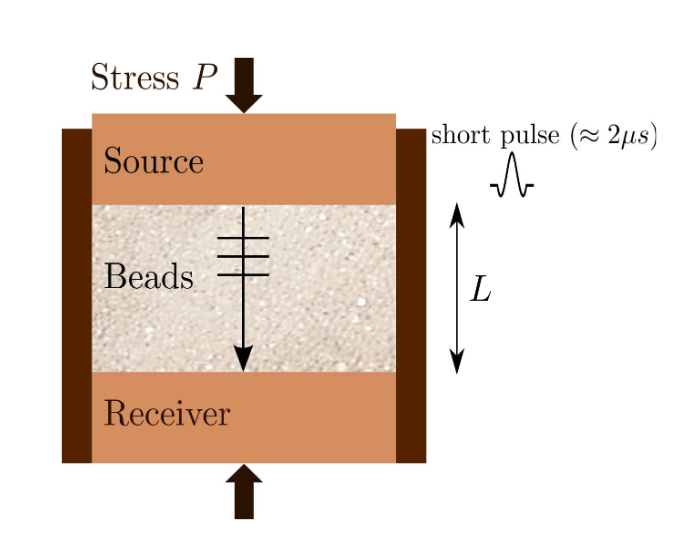
Acoustic measurements are performed using a pulse transmission through granular media under stress. The beads are poured by rain deposition into a rigid cell of inner diameter $30 \text{mm}$.

A plane-wave source (longitudinal) transducer of diameter $30 \text{mm}$ is placed on the top of the cell and the wave transmission is detected by a similar transducer on the bottom; both the source and the detector are in direct contact with the beads (Fig 1). Before the ultrasonic measurements, two cycles of loading and unloading are performed to improve the reproducibility of measurements.

声学测量采用脉冲传输方式，通过受力的颗粒介质进行。珠子通过下雨沉积倒入一个内径为 30 毫米的硬质池中。

一个直径为 30 毫米的平面波源（纵向）传感器被放置在样品池的顶部，波的传输由底部的类似传感器检测；声源和探测器都与珠子直接接触（图 1）。在进行超声波测量之前，先进行两次加载和卸载循环，以提高测量的重现性。

Various granular samples are investigated in this study. Table I summarizes the main characteristics like constitutive material (glass, PMMA or steel), mean size of beads, polydispersity and sphericity. The beads with a mean diameter larger than 1mm have a good spherical shape and a low polydispersity, while the smaller ones present sometimes a non-spherical shape (e.g., partial coalescence of two beads) and higher polydispersity.

The use of polymeric beads, e.g., PMMA, allows us to evaluate the effect of dissipation mechanisms on the coherent wavefront. Indeed, by measuring the absorption time (not shown here) from the time-resolved intensity profile of scattered waves [20, 21], we infer a wave dissipation four times larger in PMMA beads than in glass beads at 300kHz, due to the viscoelastic loss.

本研究调查了各种颗粒样本。表 I 总结了构成材料（玻璃、聚甲基丙烯酸甲酯或钢）、珠子平均尺寸、多分散性和球形度等主要特征。平均直径大于 1 毫米的珠子具有良好的球形和较低的多分散性，而较小的珠子有时会呈现非球形（例如两个珠子部分凝聚）和较高的多分散性。

Impulse response and wave velocity measurement

To obtain the impulse response of the coherent compressional wave in granular media, we may deconvolve the signals transmitted through the media by the signal $S$ sent by the source transducer. Fig. 2 shows an example of the measured signal and deconvolved one (first part). The source signal $S$ (inset of Fig. 2b) is obtained by putting the source against the detector via a coupling film. The deconvolution calculation, based on FFT, is performed on the frequency range $[1\text{kHz} − 900\text{kHz}]$.

As in [14], we characterize the impulse response of the coherent signal by the arrival times associated to three particular points: the peak $A_{1} (t_{1})$, the first arrival at $10\text{%}$ of the peak $(t_{0})$, and the first zero crossing ($t_{2}$). Complementary measurements of pulse transmission were also performed in a reference medium, i.e. water filling up the above cell (waterproof) in which the shape of received signal does not evolve significantly as the distance sourcereceiver increases. This observation indicates that the source transducer does generate a quasi-plane wave and the effect of edge waves are negligible in our experiments.

为了获得相干压缩波在颗粒介质中的脉冲响应，我们可以用源传感器发送的信号 $S$ 对通过介质传输的信号进行解卷积。图 $2$ 显示了测量信号和解卷积信号（第一部分）的示例。声源信号 $S$（图 2b 插图）是通过耦合膜将声源对准探测器得到的。基于 FFT 的解卷积计算是在 $[1\text{kHz} - 900\text{kHz}]$ 的频率范围内进行的。

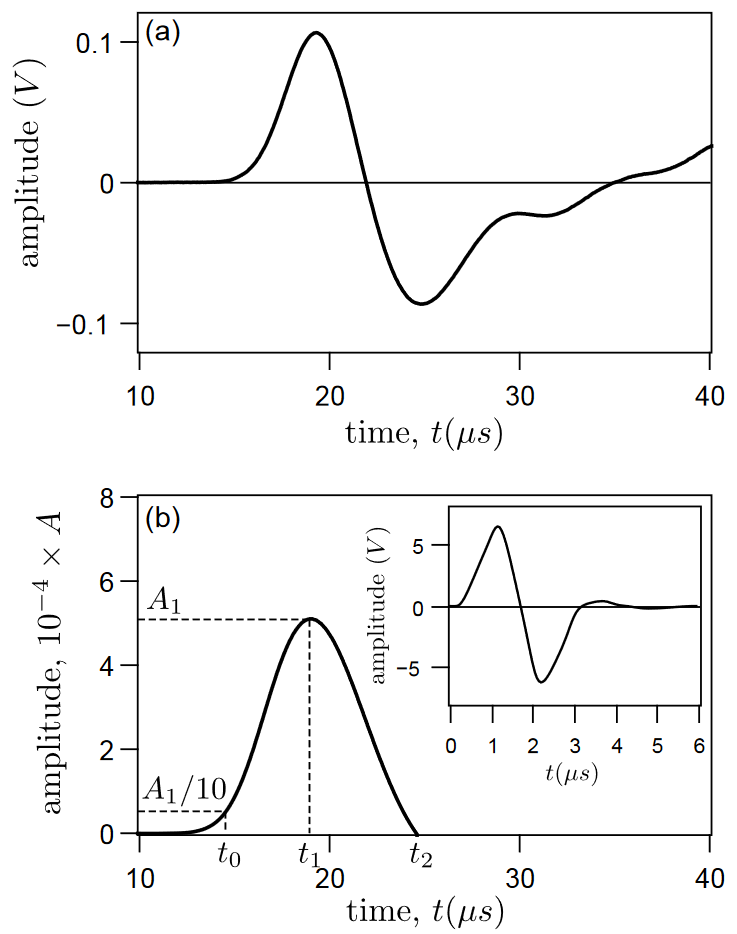
(a) Measured pulse of a compressional wave measured in a glass bead packing of d = 0.715 mm, under stress P = 995 kPa and at a distance L = 21.7 mm. (b) The deconvolved pulse of the transmitted signal (first part), by a reference signal from the source traducer (inset).

(a) 在应力 $P = 995 \text{kPa}$ 和距离 $L = 21.7 \text{mm}$ 的情况下，在 $d = 0.715 \text{mm}$ 的玻璃珠填料中测量到的压缩波脉冲。(b) 透射信号的解卷积脉冲（第一部分），以及来自信号源传感器的参考信号（插图）。

与文献$[14]$一样，我们通过与三个特定点相关的到达时间来描述相干信号的脉冲响应：峰值 $A_{1} (t_{1})$、首次到达峰值 $10\text{%}$ $(t_{0})$ 和首次过零 ($t_{2}$)。脉冲传输的补充测量也是在参考介质中进行的，即在上述电池（防水）中注入水，在这种介质中，接收信号的形状不会随着源接收器距离的增加而发生显著变化。这一观察结果表明，在我们的实验中，源传感器确实产生了准平面波，边缘波的影响可以忽略不计。

In pulse transmission experiments, the wave velocity may be determined via the time-of-flight method, making measurements at two different distances. If only onedistance measurement is conducted for the velocity calculation, the different time $t_0, t_1$ or $t_2$ leads obviously to different values (Fig. 3). Notice however that the velocity determined with $t_1$ is almost independent of the sourcereceiver distance, contrary to the other times used.

As shown in Fig. 3, this velocity determined under low stress may exhibit a slight increase with the distance sourcereceiver. Such discrepancy could be improved by an alternative method based on the Hilbert transform using a reference signal, for example, the source signal. Nevertheless, the difference between the velocity measured via $t_1$ and that determined by the alternative method is no more than $5\text{%}$.

在脉冲传输实验中，可以通过飞行时间法确定波速，在两个不同距离进行测量。如果只进行一次距离测量来计算速度，不同的时间 $t_0、t_1$ 或 $t_2$ 显然会导致不同的数值（图 $3$）。但请注意，与其他时间相反，用 $t_1$ 测得的速度几乎与源接收器距离无关。

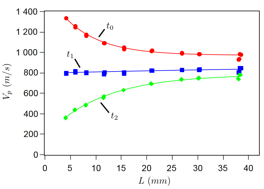
如图 $3$ 所示，在低应力条件下测定的这一速度可能会随着源接收器距离的增加而略有增加。这种差异可以通过使用参考信号（例如源信号）进行基于 Hilbert 变换的替代方法来改善。尽管如此，通过 $t_1$ 测得的速度与替代方法确定的速度之间的差异不会超过 $5\text{%}$。

The wave velocity measurement has been extensively used to study the nonlinear elasticity of stressed granular media, see, e.g., [4, 6]. Figure 4a shows that as the confining pressure is decreased, there is an increase of the time-of-flight, a decay of the pulse amplitude and a broadening of the pulse. However, by rescaling the time $t/t_1$ and the amplitude $A/A_1$ axes, we find that almost all responses collapse (Fig. 4b), indicating that the coherent wavefront are mainly governed by the time scale $t/t_1$ or $V_{p}t$.

To evaluate the accuracy of this collapse, we compare the normalized width of the signal, $W = (t_1 − t_0)/t_1$ at high and low pressures (inset of Fig. 4). The normalized width at low pressure is always higher than that obtained at high pressure. This difference may arise from the heterogeneity of the contact force networks which is more important at lower confining pressure.

For glass bead packings, the collapse of the rescaled responses appears more effective with beads of large size, less polydisperse and more spherical whose packing structures are expected to be less disordered. These results would suggest a possible dependence of the normalized width on the amount of disorder.

波速测量已被广泛用于研究受压粒状介质的非线性弹性，见 [4, 6] 等。图 4a 显示，随着约束压力的降低，飞行时间增加，脉冲振幅衰减，脉冲变宽。然而，通过重新标定时间 $t/t_1$ 和振幅 $A/A_1$ 轴，我们发现几乎所有的响应都塌缩了（图 4b），这表明相干波前主要受时间尺度 $t/t_1$ 或 $V_{p}t$ 的支配。

为了评估这种坍缩的准确性，我们比较了高压和低压下的信号归一化宽度 $W = (t_1 - t_0)/t_1$（图 4 插图）。低压下的归一化宽度总是高于高压下的归一化宽度。这种差异可能是由于接触力网络的异质性造成的，这种异质性在较低的约束压力下更为重要。

对于玻璃珠堆积，重标定响应的坍缩对于大尺寸、不太多分散和球形的玻璃珠似乎更有效，其堆积结构的无序程度预计会更低。这些结果表明，归一化宽度可能与无序程度有关。

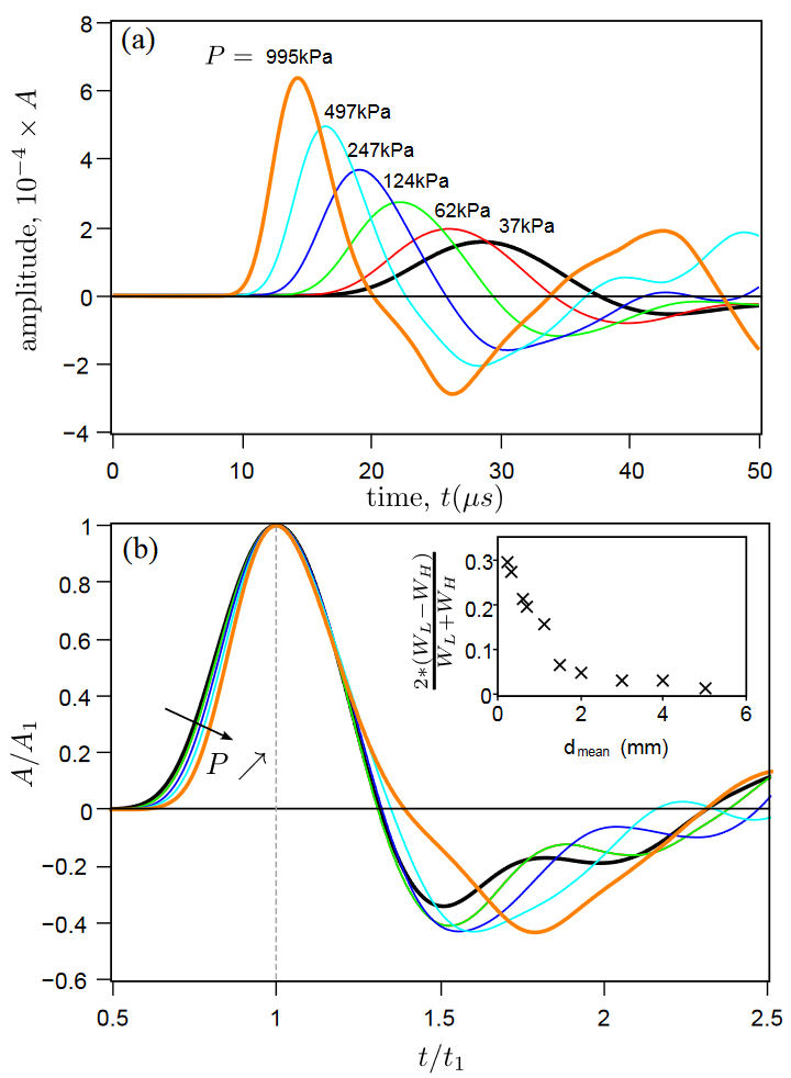
The effect of the confining pressure $P$ on the shape of the pulse signal measured at $L = 11.5 \text{mm}$. (a) Decreasing the pressure leads to an increase of the pulse width. (b) Rescaling the time axis by $t_1$ and the amplitude axis by $A_1$ leads to collapse of pulse signals. Inset: Decreasing the pressure make increase the normalized width $W$ with $W_H = W(P = 995\text{kPa})$ and $W_L = W (P = 65\text{kPa})$.

封闭压强 $P$ 对在 $L = 11.5 \text{mm}$ 处测量的脉冲信号形状的影响。(a) 压力降低导致脉冲宽度增加。(b) 时间轴按 $t_1$ 缩放，振幅轴按 $A_1$ 缩放，导致脉冲信号坍缩。插图：减小压力会增加归一化宽度 $W$，$W_H = W(P = 995\text{kPa})$ 和 $W_L = W (P = 65\text{kPa})$。

Evolution of sound pulse width

Figure 5a shows that a pulse broadening and decay with the distance of propagation through granular media. The width of the signal, $t_1 − t_0$, scales with the ratio $L/d$ as a power law with exponent of about $1/2$ or higher for beads of large size (Fig. 5b). However, if the pulse width is normalized by the propagation time $t_1$, it decreases with the propagation distance $L/d$ , according to

$$ W \approx C_{\text{W}}\left(\frac{L}{d}\right)^{-0.5} $$

where $C_{\text{W}}$ is a prefactor. Moreover, Fig. 5c shows that the data of these normalized widths are much less disperse compared to those in Fig. 5b, ranged in a greyband likely independent of the material property of beads and its mean size $d$. The data located in the upper part of this band are obtained with less spherical small beads. The results obtained from PMMA beads are very similar to those from glass beads, showing that the viscoelastic dissipation does not significantly affect measurements of the normalized pulse width.

图 5a 显示，脉冲在颗粒介质中传播的距离越远，信号越宽，衰减越大。信号宽度 $t_1 - t_0$ 与比率 $L/d$ 呈幂律关系，对于大尺寸珠子，指数约为 $1/2$ 或更高（图 5b）。但是，如果将脉冲宽度按传播时间 $t_1$ 归一化，则它会随着传播距离 $L/d$ 的增加而减小，其计算公式为

$$ W \approx C_{\text{W}}\left(\frac{L}{d}\right)^{-0.5} $$

其中 $C_{\text{W}}$ 是一个前置因子。此外，图 5c 显示，与图 5b 中的数据相比，这些归一化宽度数据的分散性要小得多，位于一个灰带中，该灰带可能与珠子的材料属性及其平均尺寸 $d$ 无关。位于灰带上部的数据是用球形较小的珠子得到的。从 PMMA 微珠得到的结果与从玻璃微珠得到的结果非常相似，这表明粘弹性耗散不会对归一化脉冲宽度的测量产生重大影响。

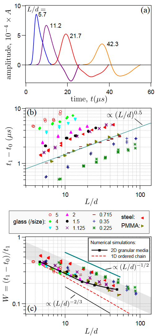
(a) Pulse broadening and decay through a glass bead packing of $d = 0.715 \text{mm}$ under stress $P = 995 \text{kPa}$. The first period (plain line) of coherent wavefront is used for the FFT analysis.

(b) Width of the pulse measured as a function of the ratio $L/d$ for different granular media under $P = 995 \text{kPa}$.

(c) Normalized pulse width $W = (t_1 − t_0)/t_1$ plotted as a function of ratio $L/d$. Numerical results in 2D disordered granular packings and 1D ordered chain simulation (dashed red line)are added here for comparison. The normalized width scales with $L$ as $W \sim C_{W}\cdot(L/d)^{−0.5}$.

(a) 在应力 $P = 995 \text{kPa}$ 条件下，脉冲展宽和衰减穿过 $d = 0.715\text{mm}$ 的玻璃珠填料。相干波面的第一周期（平直线）用于 FFT 分析。

(b) 不同颗粒介质在 $P = 995 \text{kPa}$ 条件下测量的脉冲宽度与比率 $L/d$ 的函数关系。

(c) 归一化脉冲宽度 $W = (t_1 - t_0)/t_1$ 与比率 $L/d$ 的函数关系图。这里添加了二维无序粒状堆积和一维有序链模拟的数值结果（红色虚线），以作比较。归一化宽度与 $L$ 的关系为 $W \sim C_{W}\cdot(L/d)^{-0.5}$。

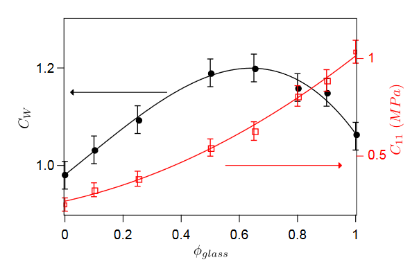
To verify whether the normalized width depends on the amount of disorder mentioned above, we investigate the evolution of the prefactor $C_{W}$ in granular packings with a mixture of glass and PMMA beads. A mixture of the beads of different nature is expected to increase the heterogeneity of stiffness and mass in the granular packings and accordingly the normalized width $W$. For a given volume fraction of glass beads $\phi_{\text{glass}}(=V_{\text{glass}}/(V_{\text{glass}} + V_{\text{pmma}}))$, we determined the prefactor $C_{W}$ by fitting the normalized widths measured for three source-receiver distances.

为了验证归一化宽度是否取决于上述无序量，我们研究了玻璃珠和 PMMA 珠混合物颗粒堆积中前因子 $C_{W}$ 的演化。不同性质珠子的混合物预计会增加颗粒堆积中刚度和质量的异质性，从而增加归一化宽度 $W$。对于给定的玻璃珠体积分数 $\phi_{\text{glass}}(=V_{\text{glass}}/(V_{\text{glass}} + V_{\text{pmma}}))$，我们通过拟合三个源-接收器距离测量的归一化宽度来确定前置因子 $C_{W}$。

Figure $6$ shows the evolution of prefactor $C_{W}$ as a function of the glass beads volume fraction $\phi_{\text{glass}}$. As expected, $C_{W}$ versus $\phi_{\text{glass}}$ presents a maximum. Instead, the elastic longitudinal modulus $C_{11}$ given by $C_{11}=\rho_{m}V_{p}^{2}$ with $\rho_{m}$ the packing density of the granular mixture, increases monotonically with the volume fraction of glass beads.

图 $6$ 显示了前因子 $C_{W}$ 与玻璃珠体积分数 $\phi_{\text{glass}}$ 的函数关系。正如预期的那样，$C_{W}$ 与 $\phi_{\text{glass}}$ 的关系呈现出最大值。相反，由 $C_{11}=\rho_{m}V_{p}^{2}$ （$\rho_{m}$ 为颗粒混合物的堆积密度）给出的弹性纵向模量 $C_{11}$，随着玻璃微珠体积分数的增加而单调增加。

Attenuation measurement by FFT

To identify the origin of the pulse broadening, we investigate the wave attenuation and velocity dispersion in frequency domain. By a FFT analysis of coherent wavefronts measured at different source-receiver distances, it is possible to determine the wave attenuation $\alpha$ and velocity dispersion as a function of frequency $\omega$.

As detailed elsewhere, the dispersion of the phase velocity is quite small in the range of frequency used here. Figures 7a and b show respectively the spectra associated with the pulses detected at different distances $L$ (Fig. 5a) and the attenuation $\alpha$ deduced from the ratio of spectra. For guidance, different scaling of attenuation on frequency ($\omega, \omega^{2}$ and $\omega^{4}$) are recalled. We discuss later in Section III C the possible mechanisms of wave attenuation.

为了确定脉冲展宽的原因，我们研究了频域中的波衰减和速度频散。通过对不同声源-接收器距离测量的相干波前进行 FFT 分析，可以确定波衰减 $\alpha$ 和速度频散作为频率 $\omega$ 的函数。

正如其他地方详述的那样，在这里使用的频率范围内，相位速度的频散相当小。图 7a 和 b 分别显示了在不同距离 $L$（图 5a）探测到的脉冲相关光谱，以及根据光谱比推导出的衰减 $\alpha$。为便于指导，我们回顾了衰减在频率上的不同比例（$\omega, \omega^{2}$ 和 $\omega^{4}$）。我们将在第三节 C 部分讨论波衰减的可能机制。

SIMULATION AND MODELING

Despite the lack of theoretical models accurately describing the sound propagation and scattering in granular media, we seek to explain our main experimental observations by the simplified numerical simulations and the general models of elastic wave scattering in random media.

尽管缺乏精确描述声音在颗粒介质中传播和散射的理论模型，我们还是试图通过简化的数值模拟和随机介质中弹性波散射的一般模型来解释我们的主要实验观察结果。

Pulse broadening versus dispersion relationship

We here consider two distinct mechanisms leading to the pulse broadening, i.e., wave attenuation $\alpha(\omega)=k’’(\omega)$ and velocity dispersion $V(\omega)=\omega/k’(\omega)$ where $k(\omega) = k’(\omega) + ik’’(\omega)$ is the complex wave number. To this end, we investigate the propagation of a plane wave $a(x,t)$ along $x$, related to its inverse Fourier transform $\widetilde{a}$ by

$$ a(x,t) = \frac{1}{2\pi}\int_{-\infty}^{+\infty}e^{-i\omega t}A(\omega)e^{ik(\omega)x}\mathrm{d}\omega $$

with $\widetilde{a} = A(\omega)e^{ik(\omega)x}$. For a Dirac-like pulse propagation, one has $A(\omega) = 1$. Two properties of the Fourier transform are recalled which are useful for the following discussions: (i) translation: if $g(t) = f(t − t_{1})$, then $\widetilde{g}(\omega) = e^{i\omega t_{1}}\widetilde{f}(\omega)$; (ii) scaling: if $g(t) = f(at)$, then $\widetilde{g}(\omega) = \left|\frac{1}{a}\right|\widetilde{f}\left(\frac{\omega}{a}\right)$.

在这里，我们考虑了导致脉冲展宽的两种不同机制，即波衰减 $\alpha(\omega)=k’’(\omega)$ 和速度色散 $V(\omega)=\omega/k’(\omega)$ 其中，$k(\omega) = k’(\omega) + ik’’(\omega)$ 是复波数。为此，我们研究了平面波 $a(x,t)$ 沿 $x$ 的传播，它与逆傅里叶变换 $\widetilde{a}$ 的关系是

$$ a(x,t) = \frac{1}{2\pi}\int_{-\infty}^{+\infty}e^{-i\omega t}A(\omega)e^{ik(\omega)x}\mathrm{d}\omega $$

其中 $\widetilde{a} = A(\omega)e^{ik(\omega)x}$。对于类 Dirac 的脉冲传播，有 $A(\omega) = 1$。我们回顾了傅立叶变换的两个特性，它们对下面的讨论非常有用：(i) 平移：如果 $g(t) = f(t - t_{1})$，那么 $\widetilde{g}(\omega) = e^{i\omega t_{1}}\widetilde{f}(\omega)$; (ii) 缩放：如果 $g(t) = f(at)$, 那么 $\widetilde{g}(\omega) = \left|\frac{1}{a}\right|\widetilde{f}\left(\frac{\omega}{a}\right)$.

Dirac-like pulse propagation

狄拉克脉冲引申自量子力学中的 Dirac Delta 函数, 在 $t = 0$ 处确定最大值, 并且在其余时间均为 $0$. 这意味着, 某个信号/波包的传播特性类似于 Dirac 脉冲, 传播过程中保持形状不变或者几乎不变, 可能会伴随着微小的扭曲或者展宽.

We first study the effect of the velocity dispersion $V(\omega)=\omega/k’(\omega)$ on the pulse broadening in a 1D massspring chain composed of identical spheres of radius $R$. There is no attenuation in such a system $(k’’ = 0)$ and the dispersion relationship is given by $k=(1/R)\sin^{-1}{\left(\frac{\omega R}{V}\right)}$ with $V$ the longitudinal wave velocity in the long wavelength limit. If the wavelength is long enough, the wavenumber can be approximated by $k = \frac{\omega}{c} + \frac{1}{6}\left(\frac{\omega}{c}\right)^{3}R^{2}$.

我们首先研究了速度色散 $V(\omega)=\omega/k’(\omega)$ 对由半径为 $R$ 的相同球体组成的一维质量弹簧链中脉冲展宽的影响。在这样的系统中不存在衰减($k’’=0$)，其色散关系为：$k=(1/R)\sin^{-1}{\left(\frac{\omega R}{V}\right)}$，其中 $V$ 为长波长极限的纵波速度。如果波长足够长，则波数可以用 $k = \frac{\omega}{c} + \frac{1}{6}\left(\frac{\omega}{c}\right)^{3}R^{2}$ 来近似.

And the Fourier transform of the signal will be given by $e^{i\left(\frac{\omega}{V}x + \frac{1}{6}\left(\frac{\omega}{V}\right)^{3}R^{2}x\right)} = e^{i\omega t_{1}}e^{i\left(\frac{1}{3}\left(\frac{\omega}{\omega_{1}}\right)^{3}\right)}$ with $t_{1} = \frac{x}{V}$ and $\omega_{1} = \left(\frac{2V^{3}}{R^{2}x}\right)^{1/3}$. The first term $e^{i\omega t_{1}}$ can be Fourier transformed using the translation property, and the second one $e^{i\left(\frac{1}{3}\left(\frac{\omega}{\omega_{1}}\right)^{3}\right)}$ corresponds to the Fourier transform of the Airy function $Ai(−x)$ scaled by the pulsation $\omega_{1}$.

信号的傅立叶变换为 $e^{i\left(\frac{\omega}{V}x + \frac{1}{6}\left(\frac{\omega}{V}\right)^{3}R^{2}x\right)} = e^{i\omega t_{1}}e^{i\left(\frac{1}{3}\left(\frac{\omega}{\omega_{1}}\right)^{3}\right)}$ 其中 $t_{1} = \frac{x}{V}$ 和 $\omega_{1} = \left(\frac{2V^{3}}{R^{2}x}\right)^{1/3}$.第一个项 $e^{i\omega t_{1}}$ 可以利用平移性质进行傅里叶变换，第二个项 $e^{i\left(\frac{1}{3}\left(\frac{\omega}{\omega_{1}}\right)^{3}\right)}$ 对应于由脉冲 $\omega_{1}$ 缩放的 Airy 函数 $Ai(-x)$ 的傅里叶变换。

As shown in $[14]$, the resultant temporal signal can be written as, $a(x,t) = \omega_{1}Ai(\omega_{1}(t_{1}-t)) = \omega_{1}Ai(\omega t_{1}\cdot\frac{t_{1}-t}{t_{1}})$. With the rescaled time axis $(t_{1} − t)/t_{1}$, the normalized width of the signal is then given by $W \sim (\omega_{1}t_{1})^{-1} = \left(\frac{R^{2}}{2x^{2}}\right)^{1/3}\propto x^{-2/3}$ namely,

$$ W \propto L^{-2/3} $$

which implies a pulse broadening $(t_{1}-t_{0}) \sim Wt_{1} \sim L^{1/3}$, as previously found.

如 $[14]$ 所示，由此产生的时间信号可以写成：$a(x,t) = \omega_{1}Ai(\omega_{1}(t_{1}-t)) = \omega_{1}Ai(\omega t_{1}\cdot\frac{t_{1}-t}{t_{1}})$ 。由于时间轴为 $(t_{1} - t)/t_{1}$ ，信号的归一化宽度为 $W \sim (\omega_{1}t_{1})^{-1}=\left(\frac{R^{2}}{2x^{2}}\right)^{1/3}\propto x^{-2/3}$ 即可.

We secondly examine a pulse propagation in a 1D random medium where the phase velocity $V = \omega/k’$ is constant, dispersionless. However, there is an attenuation given by $\alpha = k’’(\omega) = [\sigma_{K}^{2}L_{c}^{n-1}]\left(\frac{\omega}{V}\right)^{n}$ with $n$ an integer; the underlying physics (and the parameters in the bracket) of such system is detailed in §III C below. The Fourier transform of the temporal signal is then $\widetilde{a}(\omega) = e^{ik’x}e^{-k’’ x} = e^{i\omega t_{1}}e^{-\left(\frac{\omega}{\omega_{1}}\right)^{n}}$ with $t_{1} = \frac{x}{V}$ and $\omega_{1} = \left(\frac{V^{n}}{\sigma_{K}^{2}L_{c}^{n-1}x}\right)^{1/n}$.

其次，我们将研究脉冲在一维随机介质中的传播，在这种介质中，相速度 $V = \omega/k’$ 是恒定的、无色散的。然而，存在一个衰减为 $\alpha = k’’(\omega) = [\sigma_{K}^{2}L_{c}^{n-1}]\left(\frac{\omega}{V}\right)^{n}$，其中 $n$ 为整数；该系统的基本物理原理（以及括号中的参数）详见下文§III C。时间信号的傅立叶变换为 $\widetilde{a}(\omega) = e^{ik’x}e^{-k’’{x}} = e^{i\omega t_{1}}e^{-\left(\frac{\omega}{\omega_{1}}\right)^{n}}$ 且 $t_{1} = \frac{x}{V}$, 以及 $\omega_{1} = \left(\frac{V^{n}}{\sigma_{K}^{2}L_{c}^{n-1}x}\right)^{1/n}$.

By considering the properties of the Fourier transform, the temporal signal is $a(x,t) = \omega_{1}s(\omega_{1}(t-t_{1}))$ where the function $s$ is the inverse Fourier transform of $e^{-\omega^{n}}$. With the rescaled time axis $(t_{1} −t)/t_{1}$, the normalized width of the signal is then $W \sim (\omega_{1}t_{1})^{-1}=(\sigma_{K})^{\frac{2}{n}}\left(\frac{L_{c}}{x}\right)^{\frac{n-1}{n}}$. In 1D randomly layered media, one has $n = 2$ (see details below in section IIIC) leading to $\alpha \sim \omega^{2}$ and $W$ at $(x = L)$

$$ W \propto L^{-1/2} $$

考虑到傅立叶变换的特性，时间信号为 $a(x,t) = \omega_{1}s(\omega_{1}(t-t_{1}))$ 其中函数 $s$ 是 $e^{-\omega^{n}}$ 的逆傅立叶变换。通过重标度时间轴 $(t_{1} -t)/t_{1}$，信号的归一化宽度为 $W \sim (\omega_{1}t_{1})^{-1}=(\sigma_{K})^{\frac{2}{n}}\left(\frac{L_{c}}{x}\right)^{\frac{n-1}{n}}$。在一维随机分层介质中，有 $n = 2$（详见下文第 IIIC 节），导致 $\alpha \sim \omega^{2}$ 和在 $(x = L)$的 $W$.

$$ W \propto L^{-1/2} $$

Simulations in 1D chains of elastic lattices

The use of normalized variables allows us to compare our experimental results to numerical simulations. As shown in Fig. 5c, the numerical results obtained in disordered 2D granular media compare quite well with our experimental results.

Moreover, the velocity dispersion in 1D ordered chains leads to a power law scaling of $W$ on distance as $(L/d)^{-2/3}$(Eq. 3) as found in $[14]$. However, the normalized widths obtained in disordered packing scales with distance as $(L/d)^{-1/2}$ (similar to Eq. 4) and have also values larger than those one deduced from ordered packings.

通过使用归一化变量，我们可以将实验结果与数值模拟结果进行比较。如图 5c 所示，在无序的二维颗粒介质中得到的数值结果与我们的实验结果比较相当接近。

此外，正如 $[14]$ 中发现的那样，一维有序链中的速度分散导致 $W$ 在距离上的幂律缩放为 $(L/d)^{-2/3}$（公式 3）。然而，在无序堆积中得到的归一化宽度随距离的缩放关系为 $(L/d)^{-1/2}$ （类似于公式 4），其值也大于从有序堆积中推导出的值。

In order to evaluate the effect of scattering attenuation on the pulse broadening, we perform the simulation in a 1D disordered mass-spring chain in the presence of the correlation length similar to random media by Fouque et al. [19]. More specifically, we consider a 1D chain of mass-spring consisted of sub-chains of length $L_{i}$ and stiffness $D_{i}$ which is uniform inside each sub-chain (Fig 8a).

为了评估散射衰减对脉冲展宽的影响，我们在 Fouque 等人[19]提出的类似于随机介质的关联长度存在的一维无序质量弹簧链中进行了模拟。更具体地说，我们考虑由长度为 $L_{i}$、刚度为 $D_{i}$ 的子链组成的一维质量弹簧链，每个子链内部的刚度是均匀的（图 8a）。

Assuming an exponential distribution of the subchain length $L_{i}$,

$$ p(L_{i}) = \frac{1}{L_{0}}e^{-\frac{L_{i}}{L_{0}}} $$

we then obtain a mean length of the sub-chains equal to $L_{0}$. If the inverse of stiffness is given by $D^{-1} = \bar{D}^{-1}(1 + \nu_{D})$ with $\bar{D}^{-1}$ the mean value and $\nu_{D}$ the fluctuation uniformly distributed in the range $[−\nu_{\text{max}}, +\nu_{\text{max}}]$, we may readily verify $\langle\nu_{D}\rangle = 0$ and the variance $\langle\nu_{D}^{2}\rangle = \sigma_{D}^{2} = (\nu_{\text{max}})^{2}/3$.

To determine the correlation length associated with such a disordered chain, we compute the correlation function of the stiffness fluctuation $\langle\nu_{D}(x)\nu_{D}(x + \Delta x)\rangle$ via ensemble average between two points separated by a distance $\Delta x$. Fig 8c shows the normalized correlation function (by $\sigma_{D}^{2}$) versus $\Delta x$, calculated for the different $L_{0}$. If we defined the correlation length $L_{c}$ corresponding to a decrease of the normalized correlation to about $0.4 (\approx e^{−1})$, we deduce a correlation length $L_{c} \approx L_{0}$ from Fig 8c.

假设子链长度 $L_{i}$ 呈指数分布:

$$ p(L_{i}) = \frac{1}{L_{0}}e^{-\frac{L_{i}}{L_{0}}} $$

我们就可以得到子链的平均长度等于 $L_{0}$。如果刚度的倒数由 $D^{-1} = \bar{D}^{-1}(1 + \nu_{D})$ 给出，其中 $\bar{D}^{-1}$ 是平均值，$\nu_{D}$ 是均匀分布在 $[−\nu_{\text{max}}, +\nu_{\text{max}}]$ 范围内的波动，我们可以很容易地验证 $\langle\nu_{D}\rangle = 0$ 和方差 $\langle\nu_{D}^{2}\rangle = \sigma_{D}^{2} = (\nu_{\text{max}})^{2}/3$.

为了确定与这种无序链相关的关联长度，我们通过相隔距离为 $\Delta x$ 的两点之间的系综平均来计算刚度波动 $\langle\nu_{D}(x)\nu_{D}(x +\Delta x)\rangle$ 的关联函数。图 8c 显示了针对不同 $L_{0}$ 计算的归一化相关函数（按 $\sigma_{D}^{2}$）与 $\Delta x$ 的关系。如果我们定义相关长度 $L_{c}$ 对应于归一化相关性下降到约 $0.4 (\approx e^{-1})$ ，我们就可以推导出相关长度 $L_{c}$ 从图 8c 中我们可以推导出关联长度 $L_{c} \approx L_{0}$.

Simulations of the pulse propagation are performing by solving the eigenproblem of the linear spring system at given initial conditions. The equation of motion of the $N$ beads is given by (Fig 8b):

$$ m\ddot{u}_{j} = D_{j+1}(u_{j+1}-u_{j}) + D_{j}(u_{j-1}-u_{j}) $$

This equation can be expressed in a matrix form $m\ddot{\mathbf{u}} = \mathbf{D}\cdot\mathbf{u}$ where $\mathbf{u}$ is the displacement vector of each bead (only the translational motion is considered here), $m$ is the constant mass of beads and $\mathbf{D}$ is a $N\times N$ matrix (for simplicity $m$ and $\bar{D}$ are here set to $1$).

通过求解给定初始条件下线性弹簧系统的特征问题来模拟脉冲传播。$N$ 小珠的运动方程由（图 8b）给出:

$$ m\ddot{u}_{j} = D_{j+1}(u_{j+1}-u_{j}) + D_{j}(u_{j-1}-u_{j}) $$

这个方程可以用矩阵形式表示 $m\ddot{\mathbf{u}} = \mathbf{D}\cdot\mathbf{u}$ 其中 $\mathbf{u}$ 是每个珠子的位移矢量（这里只考虑平移运动）、$m$ 是珠子的恒定质量，$\mathbf{D}$ 是一个 $N \times N$ 的矩阵（为简单起见，$m$ 和 $\bar{D}$ 在此设为 $1$）。

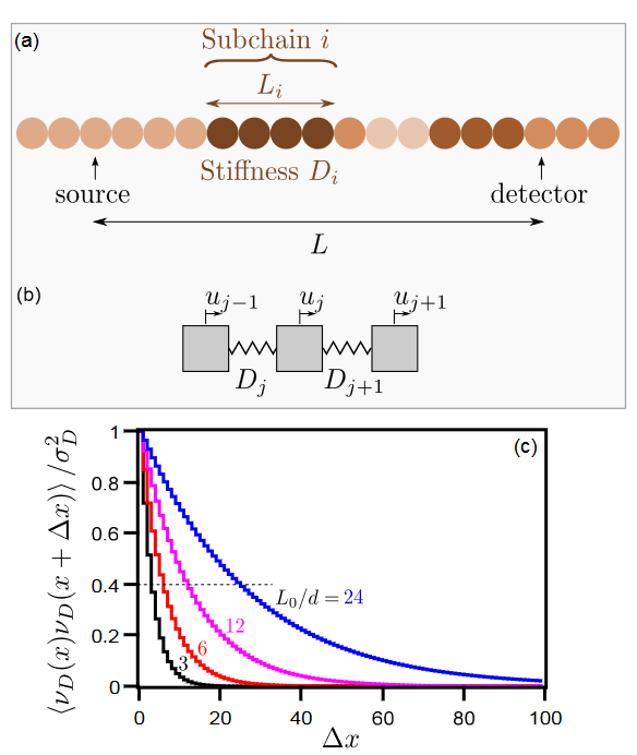
(a) Random 1D chain (see text).

(b) The interaction between the nearest neighboring beads.

(c) Auto-correlation function of the fluctuation $\nu_{D}$ of the inverse stiffness $D^{-1}$ versus separate distance $\Delta x$ for different mean lengths $L_{0}$.

(a) 随机一维链（见正文）。

(b) 最近相邻珠子之间的相互作用。

(c) 不同平均长度 $L_{0}$ 时，逆刚度 $D^{-1}$ 的波动 $\nu_{D}$ 与独立距离 $\Delta x$ 的自相关函数。

Eigenfrenquencies $\omega_{n}$ of this linear system are the square roots of the eigenvalues of the matrix $\mathbf{D}/m$. The oscillations of beads are given by the superposition of the eigenmodes: $\mathbf{u}(t) = \sum_{n}A_{n}u_{n}\cos{(\omega_{n}t)}$ where $u_{n}$ are the eigenvectors of the matrix $\mathbf{D}/m$ and the amplitudes $A_{n}$ are determined by the initial conditions.

这个线性系统的特征频率 $\omega_{n}$ 是矩阵 $\mathbf{D}/m$ 的特征值的平方根。珠子的振荡由特征模的叠加给出：$\mathbf{u}(t) = \sum_{n}A_{n}u_{n}\cos{(\omega_{n}t)}$ 其中 $u_{n}$ 是矩阵 $\mathbf{D}/m$ 的特征向量，振幅 $A_{n}$ 由初始条件决定。

To prevent the wave reflections at the edges, the source and the detector are placed in the middle of the chain. Assuming at $t = 0$ the particle displacement $u$ located at the source is equal to one, the propagation of the pulse for various sourcedetector distances $L$ is then computed with the displacement $u(t)$, averaged over $100000$ configurations.

为了防止波在边缘发生反射，源和探测器被放置在链的中间。假定在 $t = 0$ 时，位于声源处的粒子位移 $u$ 等于 1，然后根据位移 $u(t)$，计算不同声源-探测器距离 $L$ 的脉冲传播情况，并对超过 $100000$ 种构型进行平均。

Figure 9a shows the evolution of the coherent wavefront where the shape of the wavefront evolves during the propagation and tends to a Gaussian-like pulse at long distance. The normalized width of the pulse is plotted in Fig. 9b as a function of the source-detector distance for the case $\sigma_{D}=0.29$.

The variance $\sigma_{D}$ slightly makes increase the normalized width and the variation of the mean or correlation length further enhances the effect on $W$. Figure 9c depicts the pulsed wave attenuation observed in frequency domain. It scales as $\omega^{2}$ and increases with the mean length of sub-chains $L_{0}$.

图 9a 显示了相干波阵面的演变过程，波阵面的形状在传播过程中不断变化，在远距离上趋向于高斯脉冲。图 9b 中绘制的是 $\sigma_{D}=0.29$ 情况下脉冲的归一化宽度与光源-探测器距离的函数关系。

方差 $\sigma_{D}$ 会略微增加归一化宽度，而平均值或相关长度的变化会进一步增强对 $W$ 的影响。图 9c 描述了在频域观察到的脉冲波衰减。它与 $\omega^{2}$ 成比例，并随子链平均长度 $L_{0}$ 的增加而增加。

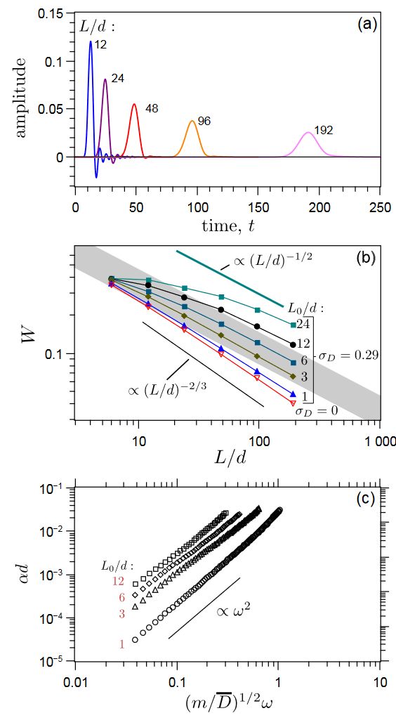
(a) Pulse broadening and decay of the coherent compressional wave propagating through a 1D chain ($\sigma_{D} = 0.29$ and $L_{0}/d = 6$).

(b) Normalized signal width as a function of $L/d$. In disordered chains, the signal is averaged on $100000$ configurations. The gray band corresponds to the experimental data dispersion (Fig. 5c is added)

(c) Attenuation (over a distance of $d$) of the coherent wave propagating through a 1D chain for $\sigma_{D} = 0.29$ and various correlation lengths.

(a) 通过一维链传播的相干压缩波的脉冲展宽和衰减（$\sigma_{D} = 0.29$，$L_{0}/d = 6$）

(b) 归一化信号宽度与 $L/d$ 的函数关系。在无序链中，信号是 $100000$ 配置的平均值。灰色条带与实验数据的离散度相对应（添加了图 5c）

(c) 在 $\sigma_{D} = 0.29$ 和各种相关长度条件下，相干波通过一维链传播时的衰减（距离为 $d$）。

Models of elastic wave scattering and dissipation

Finally, we compare our experimental and numerical results with the theoretical models of elastic wave propagation in random or granular media. In these scattering media, the models seek to relate the attenuation of coherent waves to the statistical properties of random media such as the elastic modulus $K$ and the density $\rho$, for instance introducing a characteristic length $L_{c}$ of the fluctuation $\nu_{K} = \Delta K^{−1}/\bar{K}^{−1}$ (see below).

最后，我们将实验和数值结果与弹性波在随机或颗粒介质中传播的理论模型进行比较。在这些散射介质中，这些模型试图将相干波的衰减与随机介质的统计特性（如弹性模量 $K$ 和密度 $\rho$）联系起来，例如引入波动 $\nu_{K} = \Delta K^{-1}/\bar{K}^{-1}$ 的特征长度 $L_{c}$ （见下文）。

Consider 1D random layers with the similar statistical properties as those investigated above in 1D disordered chains and free of dispersion and dissipation. Assuming $L_{c}\ll \lambda\ll L$ and a high level of disorder corresponding to a variance $\langle\nu_{K}^{2}\rangle = \sigma_{K}^{2} \sim 1$, Fouque et al. [19] show that the waveform of a coherent pulse tends to a Gaussian signal at long distance of propagation (Fig. 9a); it propagates at an effective velocity $\bar{V} = \sqrt{\bar{K}/\bar{\rho}}$:

$$ a(L,t) = \frac{1}{\sqrt{2\pi\omega_{L}^{2}}}e^{-\frac{(t-L/\bar{V})^{2}}{2\omega_{L}^{2}}} $$

where $\omega_{L} = (\gamma L/2\bar{V}^{2})^{1/2}$ governs the pulse width and $\gamma = \int_{0}^{\infty}\langle\nu_{K}(0)\nu_{K}(x)\rangle\mathrm{d}x = \sigma_{K}^{2}L_{c}$ is determined by the product of the variance $\sigma_{K}^{2}$ and the correlation length $L_{c}$.

Eq. 7 implies that the normalized width $W \sim \omega_{L}/(L/\bar{V})$ scales with propagation distance $L$ as $(\sigma_{K}^{2}L_{c}/L)^{1/2}$, and that the attenuation of the pulse is given by $\alpha = \gamma\left(\frac{\omega}{2V}\right)^{2}$.

考虑与上述在 1D 无序链中研究的那些具有相似统计特性的 1D 随机层，不受色散和耗散影响。假设 $L_{c}\ll \lambda\ll L$，并且高度无序对应于方差 $\langle\nu_{K}^{2}\rangle = \sigma_{K}^{2} \sim 1$，Fouque等人 [19] 表明，在传播的远距离处，相干脉冲的波形趋向于高斯信号（图9a）；它以有效速度 $\bar{V} = \sqrt{\bar{K}/\bar{\rho}}$ 传播:

$$ a(L,t) = \frac{1}{\sqrt{2\pi\omega_{L}^{2}}}e^{-\frac{(t-L/\bar{V})^{2}}{2\omega_{L}^{2}}} $$

其中 $\omega_{L} = (\gamma L/2\bar{V}^{2})^{1/2}$ 控制脉冲宽度，$\gamma = \int_{0}^{\infty}\langle\nu_{K}(0)\nu_{K}(x)\rangle\mathrm{d}x = \sigma_{K}^{2}L_{c}$ 由方差 $\sigma_{K}^{2}$ 和相关长度 $L_{c}$ 的乘积确定。

方程 7 意味着，归一化宽度 $W \sim \omega_{L}/(L/\bar{V})$ 随传播距离 $L$ 缩放为 $(\sigma_{K}^{2}L_{c}/L)^{1/2}$，而脉冲的衰减由 $\alpha = \gamma\left(\frac{\omega}{2V}\right)^{2}$ 给出.

Figure 10 depicts numerical results from simulations in disordered chains, regarding the normalized width $W$ for various source-detector distances $L/d$ as a function of a combined parameter $(\sigma_{D}L_{c}/L)^{1/2}$. More specifically, at a given distance $L$, we determine $W$ by varying the variance $\sigma_{D}$ or/and the correlation length $L_{c}$.

The stack data show that for high disorder $W$ scales as $(\sigma_{D}^{2}L_{c}/L)^{1/2}$ as predicted above, while for the weak level of disorder, i.e. $\sigma_{D}^{2}\left(\frac{L_{c}}{d}\right)\leq \left(\frac{L_{c}}{d}\right)^{-1/3}$, $W$ tends to the constant values as those determined in ordered 1D elastic chains (represented by the horizontal solid lines). In terms of the dispersion relationship for the high level of disorder, the attenuation is given by $\alpha = \sigma_{D}^{2}L_{c}k^{2}/4 \sim \omega^{2}$, consistent with the results shown in Fig. 9c.

图 10 描述了在无序链中模拟的数值结果，即不同源-探测器距离 $L/d$ 的归一化宽度 $W$ 与组合参数 $(\sigma_{D}L_{c}/L)^{1/2}$ 的函数关系。更具体地说，在给定距离 $L$ 时，我们通过改变方差 $\sigma_{D}$ 或/和相关长度 $L_{c}$ 来确定 $W$。

堆栈数据显示，对于高无序度，$W$ 的尺度为 $(\sigma_{D}^{2}L_{c}/L)^{1/2}$ ，如上文预测的那样，而对于弱无序度，即 $\sigma_{D}^{2}\left(\frac{L_{c}}{d}\right)\leq \left(\frac{L_{c}}{d}\right)^{-1/3}$, $W$ 会趋向于在有序一维弹性链中确定的恒定值（用水平实线表示）。根据高无序度的频散关系，衰减值为 $\alpha = \sigma_{D}^{2}L_{c}k^{2}/4 \sim \omega^{2}$ ，这与图 9c 中显示的结果一致。

In 3D random media without dispersion and dissipation, the attenuation may be expressed in the limit case $k^{2}\gamma L\ll 1$, by

$$ \alpha \sim \sigma_{K}^{2}L_{c}^{n-1}k^{n} \sim \omega^{n} $$

where $n = 2$ corresponds to the large scale fluctuation ($L_{c}\gg \lambda$) with a strongly anisotropic scattering, identical to the above result obtained in 1D random media (see also Fig. 9c), and $n = 4$ corresponds to the small scale fluctuation ($L_{c}\ll \lambda$) with an isotropic Rayleigh-like scattering.

在没有色散和耗散的三维随机介质中，衰减在极限情况 $k^{2}\gamma L\ll 1$ 下可表示为

$$ \alpha \sim \sigma_{K}^{2}L_{c}^{n-1}k^{n} \sim \omega^{n} $$

其中，$n = 2$ 对应的是具有强各向异性散射的大尺度波动（$L_{c}\gg \lambda$）, 与上述在一维随机介质中得到的结果相同（另见图 9c）; $n = 4$ 对应的是具有各向同性类 Rayleigh 散射的小尺度波动（$L_{c}\ll \lambda$）。

Regarding the experimental data of attenuation shown in Fig. 7 and in [28], these two mechanisms of scattering invoked here corresponding to $\alpha \sim \omega^{2}$ and $\alpha \sim \omega^{4}$, respectively, may explain qualitatively the measurements at the high-frequency range (note that the former appears more significant in the present work), due to the heterogeneous and anisotropic structure of the contact force networks. However, at the low-frequency range, we experimentally observe a different behavior of attenuation $\alpha \sim \omega^{1}$.

As mentioned before, the viscoelastic dissipation related to the particle material seems to be negligible here. Nevertheless, the wave dissipation around the bead contacts via thermoelastic relaxation might be a mechanism responsible for such kind of attenuation, as proposed by Wang and Santamarina, when the characteristic time is comparable with $\sim 1/\omega$.

关于图 7 和 [28] 中显示的衰减实验数据，这里引用的这两种散射机制分别对应于 $\alpha \sim \omega^{2}$ 和 $\alpha \sim \omega^{4}$，可以定性地解释高频范围的测量结果（注意，由于接触力网络的异质和各向异性结构，前者在本研究中显得更为重要）。然而，在低频范围，我们在实验中观察到了衰减 $\alpha \sim \omega^{1}$ 的不同行为。

如前所述，与颗粒材料有关的粘弹性耗散在这里似乎可以忽略不计。然而，正如 Wang 和 Santamarina 所提出的，当特征时间与 $\sim 1/\omega$ 相近时，通过热弹性弛豫在珠子接触点周围产生的波耗散可能是导致这种衰减的机制。

CONCLUSION

We have studied the pulse broadening of coherent sound waves propagating in granular media. The evolution of the pulse width of the coherent compressional wave is analyzed in terms of the dispersion relationship, including wave attenuation and velocity dispersion. The pulse broadening measured in various disordered bead packings reveals both a different scaling law on distance of propagation $L$ and larger values, compared to analytical and numerical results only invoking the dispersion effect as that found in ordered elastic lattices. The numerical simulations carried out in 1D disordered elastic systems composed of sub-chains show that the pulse broadening may be caused by scattering attenuation.

More specifically, the normalized pulse width $W$ by the wave propagation time scales with distance as $\propto L^{-1/2}$ instead $\propto L^{-2/3}$ due to the dispersion, and significantly depends on the product of the inverse stiffness variance $\sigma_{D}^{2}$ and the correlation length $L_{c}$. Our experimental and numerical results are consistent with theoretical models of elastic wave scattering in 1D and 3D random continuous media, suggesting a dominant attenuation mechanism $\alpha \sim \omega^{2}$ possibly due to an anisotropic-like scattering. Further works are still necessary to highlight the underlying physics of attenuation at the low-frequency range.

我们研究了在颗粒介质中传播的相干声波的脉冲展宽。我们从频散关系（包括波衰减和速度频散）的角度分析了相干压缩波脉冲宽度的演变。与只引用有序弹性晶格中的色散效应的分析和数值结果相比，在各种无序珠粒中测量到的脉冲展宽显示了不同的传播距离 $L$ 缩放规律和更大的数值。在由子链组成的一维无序弹性系统中进行的数值模拟显示，脉冲展宽可能是由散射衰减引起的。

更具体地说，波传播时间的归一化脉冲宽度 $W$ 与距离的比例为 $\propto L^{-1/2}$ 而不是 $\propto L^{-2/3}$，这是由色散引起的，并且很大程度上取决于反刚度方差 $\sigma_{D}^{2}$ 和相关长度 $L_{c}$ 的乘积。我们的实验和数值结果与一维和三维随机连续介质中弹性波散射的理论模型相一致，表明可能由于各向异性的散射，$\alpha \sim \omega^{2}$ 是一种主要的衰减机制。要突出低频衰减的基本物理原理，仍需进一步研究。

For future studies, the effects of disorder via mass or spring fluctuations found by numerical simulation in 1D chains need to be investigated in 2D or 3D disordered elastic networks. In these cases, the additional topological disorder appears and the absence of a reference medium prevents actually the analytical model of sound propagation. Numerical simulation may help to better understand the elastic wave propagating in granular media.

在未来的研究中，需要在二维或三维无序弹性网络中研究一维链中通过数值模拟发现的质量或弹簧波动产生的无序效应。在这些情况下，会出现额外的拓扑无序，而且由于缺乏参考介质，实际上无法使用声音传播的分析模型。数值模拟有助于更好地理解在颗粒介质中传播的弹性波。