本页面内容学习自关济寰的个人博客画转角石墨烯示意图(附 Python 代码).
因为正在研究转角双层石墨烯, 并且个人常常使用 Matlab 来绘制图像, 对于 Python 的数值计算使用十分欠缺, 因此抄录于此以进行学习.
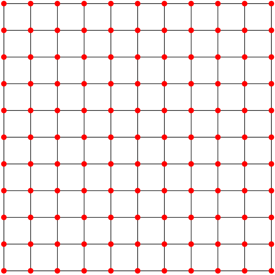
简单正方晶格
#绘制简单正方晶格
#使用conda切换至cmp环境(conda activate cmp)
import numpy as np

def main():
    x_array = np.arange(-5,5.1)
    y_array = np.arange(-5,5.1)
    coordinates=[]
    for x in x_array:
        for y in y_array:
            coordinates.append([x,y])
    plot_dots(coordinates)

def plot_dots(coordinates):
    import matplotlib.pyplot as plt
    fig,ax = plt.subplots(figsize=(9,9))
    plt.subplots_adjust(left=0.05,bottom=0.05,right=0.95,top=0.95)
    plt.axis('off')
    for i1 in range(len(coordinates)):
        for i2 in range(len(coordinates)):
            if np.sqrt((coordinates[i1][0]-coordinates[i2][0])**2+(coordinates[i1][1]-coordinates[i2][1])**2)<1.1:
                ax.plot([coordinates[i1][0],coordinates[i2][0]],[coordinates[i1][1],coordinates[i2][1]],'-k',linewidth=1)
    for i in range(len(coordinates)):
        ax.plot(coordinates[i][0],coordinates[i][1],'ro',markersize=10)
    plt.savefig('simple-square-lattice.eps')
    plt.show()

if __name__ == '__main__':
    main()
运行结果:
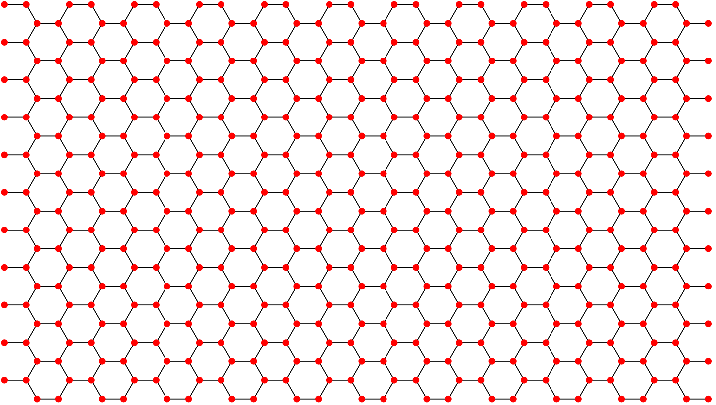
单层石墨烯
import numpy as np

def main():
    x_array = np.arange(-5,5.1)
    y_array = np.arange(-5,5.1)
    coordinates=[]
    for x in x_array:
        for y in y_array:
            coordinates.append([0+x*3,0+y*np.sqrt(3)])
            coordinates.append([1+x*3,0+y*np.sqrt(3)])
            coordinates.append([-1/2+x*3,np.sqrt(3)/2+y*np.sqrt(3)])
            coordinates.append([-3/2+x*3,np.sqrt(3)/2+y*np.sqrt(3)])
    plot_dots(coordinates)

def plot_dots(coordinates):
    import matplotlib.pyplot as plt
    x_range = max(np.array(coordinates)[:,0])-min(np.array(coordinates)[:,0])
    y_range = max(np.array(coordinates)[:,1])-min(np.array(coordinates)[:,1])
    fig,ax = plt.subplots(figsize=(9*x_range/y_range,9))
    plt.subplots_adjust(left=0.05,bottom=0.05,right=0.95,top=0.95)
    plt.axis('off')
    for i1 in range(len(coordinates)):
        for i2 in range(len(coordinates)):
            if np.sqrt((coordinates[i1][0]-coordinates[i2][0])**2+(coordinates[i1][1]-coordinates[i2][1])**2)<1.1:
                ax.plot([coordinates[i1][0],coordinates[i2][0]],[coordinates[i1][1],coordinates[i2][1]],'-k',linewidth=1)
    for i in range(len(coordinates)):
        ax.plot(coordinates[i][0],coordinates[i][1],'ro',markersize=8)
    plt.savefig('single-layer-graphene.eps')
    plt.show()

if __name__ == '__main__':
    main()
运行结果:
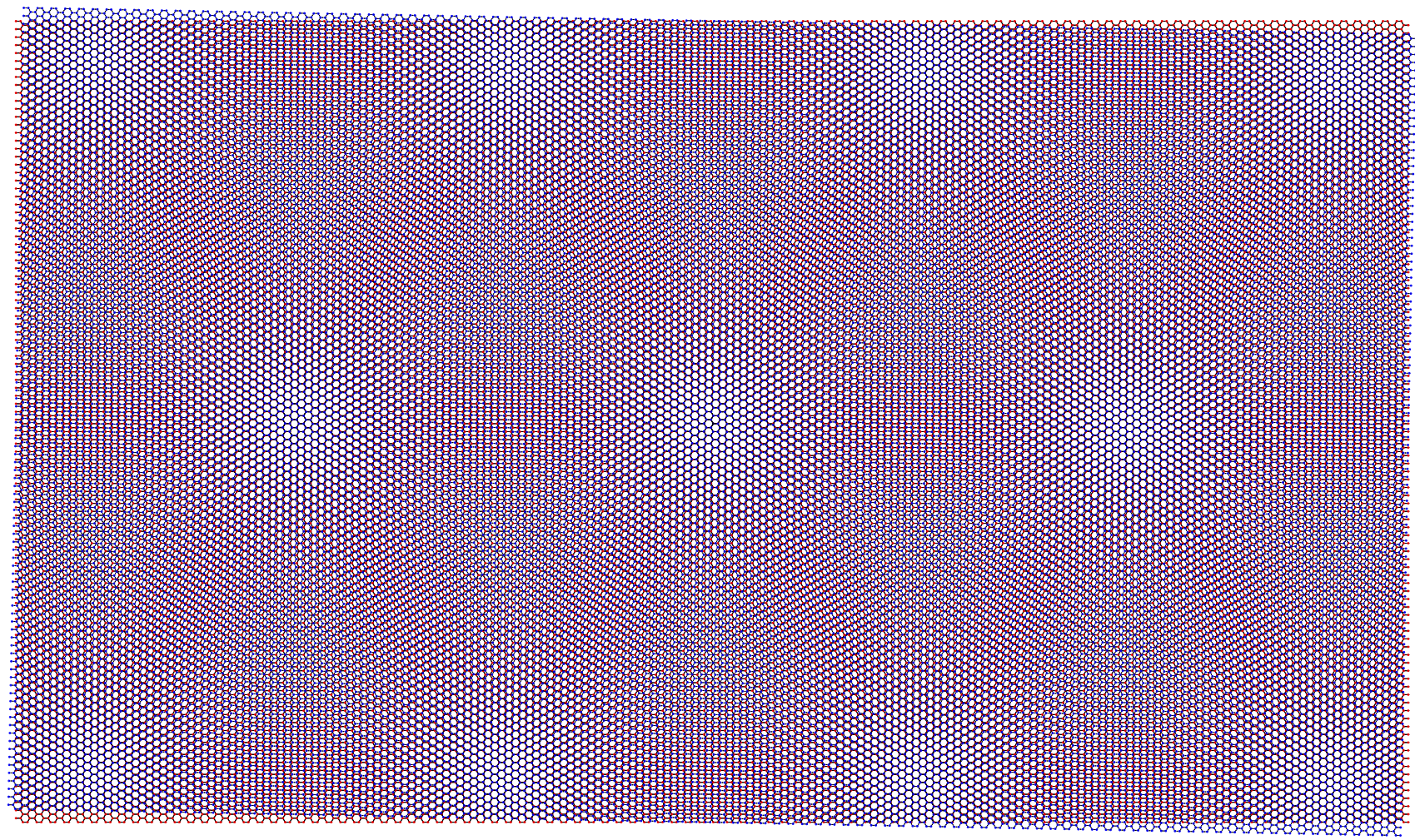
转角双层石墨烯
import numpy as np
import copy
import matplotlib.pyplot as plt
from math import *

def main():
    x_array = np.arange(-50,50.1)
    y_array = np.arange(-50,50.1)
    coordinates=[]
    for x in x_array:
        for y in y_array:
            coordinates.append([0+x*3,0+y*np.sqrt(3)])
            coordinates.append([1+x*3,0+y*np.sqrt(3)])
            coordinates.append([-1/2+x*3,np.sqrt(3)/2+y*np.sqrt(3)])
            coordinates.append([-3/2+x*3,np.sqrt(3)/2+y*np.sqrt(3)])
    x_range1 = max(np.array(coordinates)[:,0])-min(np.array(coordinates)[:,0])
    y_range1 = max(np.array(coordinates)[:,1])-min(np.array(coordinates)[:,1])

    theta = -1.1/180*pi
    rotation_matrix=np.zeros((2,2))
    rotation_matrix[0][0]= np.cos(theta)
    rotation_matrix[0][1]=-np.sin(theta)
    rotation_matrix[1][0]= np.sin(theta)
    rotation_matrix[1][1]= np.cos(theta)
    coordinates2 = copy.deepcopy(coordinates)
    for i in range(len(coordinates)):
        coordinates2[i] = np.dot(rotation_matrix,coordinates[i])
    x_range2 = max(np.array(coordinates2)[:,0])-min(np.array(coordinates2)[:,0])
    y_range2 = max(np.array(coordinates2)[:,1])-min(np.array(coordinates2)[:,1])

    x_range = max(x_range1,x_range2)
    y_range = max(y_range1,y_range2)
    fig,ax=plt.subplots(figsize=(9*x_range/y_range,9))
    plt.subplots_adjust(left=0.05,bottom=0.05,right=0.95,top=0.95)
    plt.axis('off')
    plot_dots_1(ax,coordinates)
    plot_dots_2(ax,coordinates2)
    plot_dots_0(ax,[[0,0]])
    plt.savefig('twisted-bilayer-graphene.eps')
    plt.show()

def plot_dots_0(ax,coordinates):
    for i in range(len(coordinates)):
        ax.plot(coordinates[i][0],coordinates[i][1],'ko',markersize=0.5)

def plot_dots_1(ax,coordinates):
    for i1 in range(len(coordinates)):
        for i2 in range(len(coordinates)):
            if np.sqrt((coordinates[i1][0]-coordinates[i2][0])**2+(coordinates[i1][1]-coordinates[i2][1])**2)<1.1:
                ax.plot([coordinates[i1][0],coordinates[i2][0]],[coordinates[i1][1],coordinates[i2][1]],'-k',linewidth=0.2)
    for i in range(len(coordinates)):
        ax.plot(coordinates[i][0],coordinates[i][1],'ro',markersize=0.5)

#相比于plot_dots_1只是改变了颜色,其余部分完全相同
def plot_dots_2(ax,coordinates):
    for i1 in range(len(coordinates)):
        for i2 in range(len(coordinates)):
            if np.sqrt((coordinates[i1][0]-coordinates[i2][0])**2+(coordinates[i1][1]-coordinates[i2][1])**2)<1.1:
                ax.plot([coordinates[i1][0],coordinates[i2][0]],[coordinates[i1][1],coordinates[i2][1]],'--k',linewidth=0.2)
    for i in range(len(coordinates)):
        ax.plot(coordinates[i][0],coordinates[i][1],'bo',markersize=0.5)

if __name__ == '__main__':
    main()
运行结果:
可以看到, 在1.1°(也就是计算提出的第一魔转角)下的转角双层石墨烯体现出了摩尔超晶格现象.